EP0789329A2 - Meshes with variable resolution - Google Patents
Meshes with variable resolution Download PDFInfo
- Publication number
- EP0789329A2 EP0789329A2 EP97100126A EP97100126A EP0789329A2 EP 0789329 A2 EP0789329 A2 EP 0789329A2 EP 97100126 A EP97100126 A EP 97100126A EP 97100126 A EP97100126 A EP 97100126A EP 0789329 A2 EP0789329 A2 EP 0789329A2
- Authority
- EP
- European Patent Office
- Prior art keywords
- mesh
- meshes
- vertex
- representation
- geomorph
- Prior art date
- Legal status (The legal status is an assumption and is not a legal conclusion. Google has not performed a legal analysis and makes no representation as to the accuracy of the status listed.)
- Granted
Links
Images


Classifications
-
- G—PHYSICS
- G06—COMPUTING; CALCULATING OR COUNTING
- G06T—IMAGE DATA PROCESSING OR GENERATION, IN GENERAL
- G06T9/00—Image coding
- G06T9/001—Model-based coding, e.g. wire frame
-
- G—PHYSICS
- G06—COMPUTING; CALCULATING OR COUNTING
- G06T—IMAGE DATA PROCESSING OR GENERATION, IN GENERAL
- G06T17/00—Three dimensional [3D] modelling, e.g. data description of 3D objects
- G06T17/20—Finite element generation, e.g. wire-frame surface description, tesselation
Definitions
- This invention relates generally to geometric modeling using polygonal meshes for computer graphics, and more particularly relates to techniques for optimizing display, storage and transmission of varying level of detail polygonal mesh models.
- a triangle mesh (e.g., example portion of a triangle mesh 82 of Fig. 6) is a piecewise linear surface consisting of triangular faces joined together along their edges.
- K is a simplicial complex specifying the connectivity of the mesh simplices (i.e., the adjacency of the vertices, edges, and faces)
- V ⁇ v 1 ,...
- ⁇ m is constructed by identifying each vertex of K with a canonical basis vector of m , and the mesh is defined as the image, ⁇ v (
- the vertices of a triangle mesh e.g., vertices 82-89 of the mesh 80 of Fig.
- surface appearance attributes other than geometry i.e., the above described simplicial complex and vertex positions tuple ( K , V )
- K , V simplicial complex and vertex positions tuple
- Discrete attributes are usually associated with faces of the mesh.
- a common discrete attribute, the material identifier determines the shader function used in rendering a face of the mesh, as well as some of the shader function's global parameters.
- a trivial shader function may involve simple look up within a specified texture map. (See, e.g., S. Upstill, The RenderMan Companion (Addison-Wesley 1990).)
- scalar attributes are often associated with a mesh, including diffuse color ( r , g , b ), normal ( n x , n y , n z ), and texture coordinates ( u , v ). More generally, these attributes specify the local parameters of shader functions defined on the mesh faces. To capture discontinuities in the scalar fields, and because adjacent faces may have different shading functions, it is common to associate scalar attributes not with vertices of a mesh, but with its corners. (See, e.g., Apple Computer, Inc., 3d Graphics Programming with QuickDraw 3d (Addison-Wesley 1995).) A corner is defined as a (vertex,face) tuple.
- Scalar attributes s (v,f) at a corner c (v j ,f k ) specify the shading parameters for face f at vertex v .
- a curve sequence of edges
- the curve partitions the corners into two sets; two normals are associated with the vertex, one for each of these sets.
- Mesh Simplification The meshes created by modeling and scanning systems are typically not optimized for display performance. In most applications, these initial meshes can usually be replaced by nearly indistinguishable approximations with far fewer faces, thereby improving rendering efficiency.
- the computer user e.g., graphical artist or designer
- a far better approach is to develop mesh simplification tools to automate this painstaking task. As another benefit, such tools allow porting of a single model to platforms of varying performance.
- Level-of-Detail Approximation When a detailed mesh is far from the viewer, it may occupy only a small region of the screen. Significant work must be expended to render the mesh only to have it affect a small number of pixels. Instead, a far coarser mesh (i.e., one with fewer vertices and faces) would look almost identical. To address this problem, many applications use several versions of a model at various levels of detail. A fully detailed mesh is used when the object is close; coarser approximations are substituted as the object recedes. (See, T.A. Funkhouser and C.H. Sequin, Adaptive Display Algorithm for Interactive Frame Rates During Visualization of Complex Virtual Environments , 1993 Computer Graphics Proceedings 247-254).
- a complex mesh consumes considerable time to transmit over a communication line, often many times longer than it takes to visually render images with views on the mesh.
- a mesh is transmitted over a communication line, one would like to render views that show progressively better approximations to the model as data is incrementally received.
- the simplest known approach is to render the individual triangles as they are received, but of course this looks extremely poor.
- Another prior approach is to transmit successive level-of-detail approximations, but this requires additional transmission time.
- Mesh compression A model should be stored in the smallest amount of memory or disk space. There have been two orthogonal approaches to dealing with this problem. One is to use mesh simplification, as described earlier, to reduce the number of faces in the model as much as possible while preserving its appearance. The other is mesh compression: minimizing the space taken to store the model given that a particular mesh has been selected.
- )) measures the total squared distance of the points from the mesh (i.e., a measurement along the accuracy axis 26), and the representation energy term E crep (M) c rep m penalizes the number m of vertices in M (i.e., a measurement along the conciseness axis 27).
- Hoppe93 describes minimizing the energy function E(M) using a nested optimization method having an outer loop and an inner loop.
- the method optimizes over K , the connectivity of the mesh, by randomly attempting a set of three possible mesh transformations: edge collapse, edge split, and edge swap.
- This set of transformations is complete, in the sense that any simplicial complex K of the same topological type as K can be reached through a sequence of these transformations.
- the algorithm in fact optimizes only one vertex position v s , and considers only the subset of points X that project onto the neighborhood affected by K ⁇ K '.
- E spring (M) The regularizing spring energy term is found in Hoppe93 to be most important in the early stages of the optimization.
- the optimization method therefore achieves best results by repeatedly invoking the nested optimization method described above with a schedule of decreasing spring constants ⁇ .
- Hoppe93 also demonstrates use of this mesh optimization method as a mesh simplification tool.
- an initial mesh M e.g., example initial arbitrary mesh shown in Fig. 1(a)
- a dense set of points X is sampled both at the vertices of M and randomly over its faces.
- the optimization method is then invoked with initial mesh M as the starting mesh.
- the optimization method takes different paths 34-36 through a space of possible meshes 38 and thereby can produce optimized meshes M b , M c , and M d with different trade-offs of accuracy and conciseness.
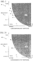
- FIG. 1(b-d) show views of three example optimized meshes M b , M c , and M d , respectively, produced from the example original arbitrary mesh (Fig. 1(a)) by the prior mesh optimization method of Hoppe93 for different values of the representation constant c rep .
- each of these records stores information associated with a vertex split, an elementary mesh transformation that adds an additional vertex to the mesh.
- the PM representation of M thus defines a continuous sequence of meshes M 0 , M 1 ,..., M n of increasing accuracy from which level-of-detail approximations with any desired complexity can be efficiently retrieved. Moreover, smooth visual transitions (geomorphs) can be efficiently constructed between any two such meshes.
- the PM representation naturally supports progressive transmission, offers a concise encoding of M itself, and supports efficient selective refinement. In short, the PM representation offers an efficient, lossless, continuous-resolution representation.
- the present invention also provides a new simplification procedure for constructing a PM representation from a given mesh M . Unlike previous simplification methods, this procedure seeks to preserve not just the geometry of the mesh surface, but also its overall appearance, as defined by the discrete and scalar attributes associated with its surface.
- the multiresolution analysis (MRA) approach of Eck95 has some similarities with the PM representation.
- the MRA approach also stores a simple base mesh, together with a stream of information that progressively adds detail back to the model.
- the MRA approach likewise produces a continuous-resolution representation from which approximations of any complexity can be extracted.
- the PM representation of the present invention has a number of differences from and advantages over the prior MRA approach.
- the MRA approach utilizes detail terms in the form of wavelets that specify transformations which recursively split the faces of a base mesh. This requires the detail terms or wavelets to lie on a domain with subdivision connectivity. As a result, each level of detail approximation, including the highest, must belong to a restricted class of meshes (those with subdivision connectivity). An arbitrary initial mesh M (with arbitrary connectivity) can only be approximately recovered to within an ⁇ tolerance, and never exactly.
- each detail record is a complete mesh refinement transformation which can produce progressive meshes ( M i ,i ⁇ n of the PM representation) having any arbitrary connectivity.
- the progressive meshes can be much better approximations geometrically of the original arbitrary mesh M than the counterpart approximating meshes of the MRA approach.
- M n the highest-detailed model in the continuous-resolution family, M n , is exactly the original arbitrary mesh M .
- the MRA approach cannot deal effectively with surface creases (curves on the surface across which the surface is not smooth), unless those creases happen to lie parametrically along edges of the base (least level of detail) mesh.
- the progressive meshes constructed according to the invention can introduce surface creases anywhere on the mesh surface and at any of the levels-of-detail.
- the PM representation can capture both continuous, piecewise-continuous, and discrete appearance attributes associated with the surface.
- attributes include diffuse color, normals, texture coordinates, material identifiers, and shader parameters.
- prior MRA schemes can use piecewise-constant basis functions, but then the resulting approximations have too many discontinuities since none of the basis functions meet continuously. (See, e.g., P. Schroder and W. Sweldens, Spherical Wavelets: Efficiently Representing Functions on the Sphere , 1995 Computer Graphics Proceedings 161-172 (the Haar wavelet basis).)
- MRA could be extended to capture discrete attributes.
- the PM representation of the invention allows geomorphs between any two levels-of-detail meshes with different discrete attributes. This is not possible with prior MRA approaches.
- Fig. 2 is a graph of accuracy versus conciseness illustrating the results of the prior mesh optimization method described in Hoppe93 for the example approximating meshes shown in Figs. 1(b-d).
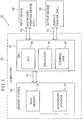
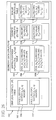
- Fig. 3 is a block diagram of a software system for viewing level of detail approximations of a mesh according to the illustrated embodiment of the invention.
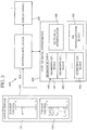
- Fig. 5 is a block diagram of a computer system that can be used to implement a method and apparatus embodying the invention for storing, transmitting and rendering views on progressive meshes using a PM representation.
- Fig. 6 is a block diagram of portions of example initial and resulting triangle meshes illustrating two inverse mesh transformations, an edge collapse operation and a vertex split operation.
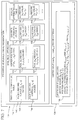
- Fig. 7 is a block diagram of a PM representation data structure for representing a succession of level-of-detail approximations of an arbitrary original mesh M according to the illustrated embodiment of the invention.
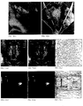
- Figs. 8(a-d) are views of three exemplary meshes ( M 0 with 50 faces in Fig. 8(a); M 75 with 200 faces in Fig. 8(b); and M 475 with 1000 faces in Figs. 8(c-d)) out of a set of progressive meshes specified in an exemplary PM representation according to the illustrated embodiment of the invention.
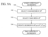
- Fig. 9(a) is a flow diagram of a method for creating geomorphs between two meshes in a PM representation according to the illustrated embodiment.
- Fig. 9(b) is a flow diagram of a method for evaluating the geomorphs created by the method of Fig. 9(a).
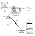
- Fig. 11 is a block diagram of a system according to the illustrated embodiment of the invention for progressively transmitting and displaying views of a three dimensional object based on the PM representation.
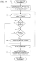
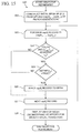
- Figs. 12(a-b) are flow charts of a transmitting method and a receiving method in the system of Fig. 11 for progressively transmitting and interactively displaying views based on the PM representation.
- Fig. 13 is a block diagram of a vertex split transformation specified in a PM representation and illustrating encoding of attributes in a vertex split record with predictive and delta encoding for mesh compression.
- Fig. 14 is a flow chart of a method according to the illustrated embodiment of the invention for selective refinement of a mesh based on the PM representation of Fig. 7.
- Fig. 15 is a flow chart of an alternative method according to the illustrated embodiment of the invention for selective refinement of a mesh based on the PM representation of Fig. 7 and using a closest living ancestor condition.
- Figs. 16(a-b) are views of exemplary meshes produced by selective refinement within a view frustum according to the methods of Figs. 14 (with 9,462 faces shown in Fig. 16(a)) and 15 (with 12,169 faces shown in Fig. 16(b)), respectively.
- Fig. 17 is a flow chart of a further modification of the methods of Figs. 13 and 14 for selective refinement of a mesh based on the PM representation of Fig. 7 which maintains more detail near silhouette edges and near the viewer.
- Figs. 18(a-b) are views of an exemplary mesh (with 7,438 faces) produced by selective refinement within a view frustum according to the method of Fig. 17.
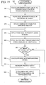
- Fig. 19 is a flow chart of a mesh simplification method according to the illustrated embodiment of the invention for constructing the PM representation of an arbitrary mesh.
- Fig. 20 is a graph of accuracy versus conciseness illustrating the results of the mesh simplification method shown in Fig. 19.
- Figs. 21(a-c) are views of a simplified mesh (Figs. 21(b-c)) produced from an exemplary arbitrary mesh (Figs. 21(a) - a mesh with regular connectivity whose vertex colors correspond to the pixels of an image) according to the simplification method of Fig. 19 and illustrating preservation of a complex scalar attribute field (i.e., color).
- Figs. 22(a-c) are views of a simplified mesh (Figs. 22(b-c)) with 10,000 faces produced from an exemplary arbitrary mesh (Fig. 22(a)) with 150,983 faces according to the simplification method of Fig. 19 illustrating preservation of a scalar attribute (radiosity).
- Figs. 23(a-d) are views of a simplified mesh (Figs. 23(c-d)) with 3,000 faces produced from an original arbitrary mesh (Figs. 23(a-b)) with 19,458 faces according to the simplification method of Fig. 19 illustrating preservation of overall appearance (including both geometry and attributes).
- Figs. 24(a-d) are views of three exemplary meshes ( M 0 with 150 faces in Fig. 24 (b); M 425 with 1000 faces in Fig. 24(c); and M 1925 with 4000 faces in Fig. 24(d)) out of a sequence of progressive meshes formed according to the simplification method of Fig. 19 from an example initial arbitrary mesh M with 13,546 faces (Fig. 24(a)).
- Figs. 25(a-c) are views of exemplary simplified meshes (each with 2000 faces) produced according to variations of the simplification method of Fig. 19 (Fig. 25(a) without E disc ; Fig. 25(b) with discontinuity curve topology fixed; and Fig. 25(c) with E disc and with discontinuity curve topology changing) illustrating preservation of the geometry of discontinuity curves.
- Fig. 26 is a block diagram of a geomorph data structure for representing a geomorph between two meshes of the PM representation of Fig. 7 which is constructed according to the geomorph construction method of Fig. 9(a).
- an operating environment for an illustrated embodiment of the present invention is a computer system 50 with a computer 52 that comprises at least one high speed processing unit (CPU) 54, in conjunction with a memory system 56, an input device 58, and an output device 60. These elements are interconnected by at least one bus structure 62.
- CPU high speed processing unit
- the illustrated CPU 54 is of familiar design and includes an ALU 64 for performing computations, a collection of registers 66 for temporary storage of data and instructions, and a control unit 68 for controlling operation of the system 50.
- the CPU 54 may be a processor having any of a variety of architectures including Alpha from Digital, MIPS from MIPS Technology, NEC, IDT, Siemens, and others, x86 from Intel and others, including Cyrix, AMD, and Nexgen, and the PowerPc from IBM and Motorola.
- the memory system 56 generally includes high-speed main memory 70 in the form of a medium such as random access memory (RAM) and read only memory (ROM) semiconductor devices, and secondary storage 72 in the form of long term storage mediums such as floppy disks, hard disks, tape, CD-ROM, flash memory, etc. and other devices that store data using electrical, magnetic, optical or other recording media.
- main memory 70 also can include video display memory for displaying images through a display device.
- the memory 56 can comprise a variety of alternative components having a variety of storage capacities.
- the input and output devices 58, 60 also are familiar.
- the input device 58 can comprise a keyboard, a mouse, a physical transducer (e.g., a microphone), etc.
- the output device 60 can comprise a display, a printer, a transducer (e.g., a speaker), etc.
- Some devices, such as a network interface or a modem, can be used as input and/or output devices.
- the computer system 50 further includes an operating system and at least one application program.
- the operating system is the set of software which controls the computer system's operation and the allocation of resources.
- the application program is the set of software that performs a task desired by the user, using computer resources made available through the operating system. Both are resident in the illustrated memory system 56.
- the computer system 50 utilizes a progressive mesh ("PM") representation to model three dimensional objects for graphics imaging as polygonal meshes at varying levels of detail.
- PM progressive mesh
- the PM representation in the illustrated embodiment operates on triangle meshes (see, discussion in the "Background and Summary of the Invention" above).
- the PM representation of the illustrated embodiment can operate with more general meshes, such as those containing n -sided faces and faces with holes, by first converting the more general mesh into a triangle mesh using conventional triangulation processes (e.g., edges are added to subdivide polygonal faces of the mesh having more than 3 sides into triangle faces).
- edge collapse transformations can be applied to the sides of polygonal faces having more than three sides to produce a triangle mesh.
- the PM representation can be generalized in alternative embodiments of the invention to operate directly with more general meshes (i.e., without prior triangulation), at the expense of more complex data structures.
- Hoppe93 (see, Background and Summary of the Invention above) describes a mesh optimization method that can be used to approximate an initial mesh M by a much simpler one.
- This mesh optimization method traverses the space of possible meshes (as discussed above with reference to the graph of Fig. 2) by successively applying a set of 3 mesh transformations: edge collapse, edge split, and edge swap.
- edge collapse transformation 110 unifies 2 adjacent vertices v s 86 and v t 89 of the mesh 80 into a single vertex v s 86' to form a resulting simpler mesh 112.
- the vertex v t 89 and the two adjacent faces ⁇ v s , v t , v l ⁇ 100 and ⁇ v s , v t , v r ⁇ 101 of the original mesh 80 vanish in the process.
- a position v s is specified for the new unified vertex 86'.
- the particular sequence of edge collapse transformations must be chosen carefully, since it determines the quality of the approximating meshes M i , i ⁇ n .
- V i ⁇ v 1 ,..., v m0 + i ⁇ , so that vertex v m0 + i + 1 is removed by ecol i .
- the position of v j in M i is denoted herein as v j i .
- a vertex split transformation denoted herein as vsplit(v s , v l , v r , v t , A) , adds near vertex v s 86' a new vertex (i.e., previously removed vertex v t 89) and two new faces (i.e., previously removed faces ⁇ v s , v t , v l ⁇ 100 and ⁇ v s , v t , v r ⁇ 101) according to the two side vertices v l 87 and v r 88.
- the transformation also updates the attributes of the mesh in the neighborhood of the transformation.
- This attribute information denoted by A , includes the positions v s and v t of the two affected vertices, the discrete attributes d ⁇ vs , vt , vl ⁇ and d ⁇ vs , vt , vr ⁇ of the two new faces, and the scalar attributes of the affected corners ( s ( vs , ⁇ ) , s ( vt , ⁇ ) , s ( vl , ⁇ vs , vt , vl ⁇ ) , and s ( vr , ⁇ vs , vt , vr ⁇ ) ).
- an arbitrary triangle mesh M therefore can be represented according to the illustrated embodiment of the invention as a data structure 130 containing a base mesh record 132 specifying the simple mesh M 0 (hereafter the "base mesh"), together with a sequence 134 of n vsplit records 136 specifying a sequence of vertex split transformations that reconstruct the arbitrary mesh M from the base mesh M 0 : M 0 vsplit 0 ⁇ M 1 vsplit 1 ⁇ ...
- vsplit n-1 ⁇ (M n M ⁇ )
- the vsplit records are parameterized as vsplit i (s i , l i , r i , A i )
- the data structure (M 0 , ⁇ vsplit 0 ,..., vsplit n-1 ⁇ ) 130 is referred to herein as a progressive mesh (PM) representation of the arbitrary mesh M .
- a significant property (referred to herein as "completeness") of the vertex split transformation is that a mesh with any arbitrary simplicial complex K A can be constructed from a mesh with a minimal simplicial complex K M of the same topological type by a sequence of one or more of the transformations.
- the four to one face split transformation used in the prior MRA approach discussed above is not complete in this sense because a sequence of these face split transformations can only construct an approximation to any arbitrary mesh from a minimal mesh of the same topological type having subdivision connectivity.) Because the vertex split transformation is complete in this sense, any arbitrary mesh can be reprented exactly using the illustrated PM representation.
- a set of one or more mesh transformations also is complete if a mesh having any arbitrary simplicial complex K A can be constructed from a minimal simplicial complex K M of the same topological type by a sequence of transformations from the set.
- vertex split transformations are specified in the sequence of records in the PM representation of the illustrated embodiment, the records in a PM representation can alternatively specify a set of mesh transformations that is complete other than the vertex split transformation.
- a set including the 4-to-1 face split transformation plus a vertex split transformation is complete and can be specified in the sequence of records in a PM representation of an alternative embodiment of the invention.
- the vertex positions table 142 contains m 0 position records 150-151 for each vertex of the base mesh M 0 with that vertex's coordinate values (x,y,z). In the illustrated vertex positions table 142, the position records 150-151 are indexed according to vertex indices associated with the indices of the base mesh M 0 .
- the simplicial complex table 140 contains face records 154-155 for each face in the base mesh M 0 with the indices of that face's vertices ⁇ v j , v k , v l ⁇ .
- This vertex information in the face records explicitly defines each face of the base mesh M 0 , and also implicitly defines the edges and corners of the base mesh M 0 .
- the base mesh record 132 can contain information which explicitly defines the edges and corners, such as records containing indices of pairs of adjacent vertices to define the edges and records containing indices of vertex index, face index tuples to define the corners.
- the face records 154-155 are indexed according to face indices associated with the faces of the base mesh M 0 .
- the discrete attributes table 144 contains records 158-159 with information (i.e., an attribute value and a face index) that defines the discrete attributes associated with the faces of the base mesh M 0 .
- the scalar attributes table 146 contains records 162-164 with information (i.e., an attribute value and a vertex index, face index tuple) that define scalar attributes associated with corners of the base mesh M 0 .
- the base mesh record 132 can contain separate attributes tables for each of multiple different discrete and scalar attributes (e.g., material identifies, shader function parameters, diffuse color, normal, texture coordinates, etc.) of the base mesh M 0 .
- the vertex split records 136 in the sequence 134 specify vertex split transformations that reconstruct the arbitrary original mesh M from the base mesh M 0 .
- the information in each of the vertex split records comprises indices of the vertices v s 86, v l 87 and v r 88 (Fig. 6); the position coordinates v s n and v t n of the vertices v s 86 and v t 89 (Fig. 6); the discrete attributes d ⁇ vs , vt , vl ⁇ and d ⁇ vs , vt , vr ⁇ of faces 100 and 101 (Fig. 6); and the scalar attributes s (vs ,.
- the vertex split records can specify the vertices v s , v l , and v r indirectly, such as by the index of a neighboring face (e.g., one including the vertices v s and v l ) and bits identifying the vertexes from those adjacent that face (e.g., identifying v s and v l out of the face's vertices, and identifying v r out of the vertices neighboring the face).
- the index of a neighboring face e.g., one including the vertices v s and v l
- bits identifying the vertexes from those adjacent that face e.g., identifying v s and v l out of the face's vertices, and identifying v r out of the vertices neighboring the face.
- the example initial arbitrary mesh M of Fig. 1(a) was simplified down to the coarse mesh M 0 170 of Fig. 8(a) (with 50 faces) using 6448 edge collapse transformations.
- the data structure of the PM representation 130 described above where the simplicial complex table 140 lists face records 154-155 containing the vertex indices of each face is used for storage purposes (e.g., storage of the progressive meshes on the hard disk of the computer system 50 of Fig. 5).
- the illustrated embodiment utilizes an edge based data structure for the simplicial complex table 140 to also encode the adjacency of faces. This allows for efficient processing of queries, such as which faces are adjacent to face f j , and which faces are adjacent to vertex v j .
- Suitable edge based data structures are well known, and include the winged-edge data structure described in K. Weiler, Edge-based Data Structures for Solid Modeling in Curved-surface Environments , IEEE CG&A 5(1):21-40 (January 1985).
- the vertex split records 136 can encode information to specify the attributes of the mesh both before and after the vertex split transformation is applied. This allows traversal of the progressive meshes sequence in both directions.
- a given mesh in the progressive mesh sequence can be either further refined by applying vertex split transformations specified in subsequent (not yet applied) vertex split records, or the mesh can be simplified by reversing the vertex split transformations specified in preceding (previously applied) vertex split records as desired.
- the added information specifies the vertex position v s in the mesh before the vertex split transformation is applied.
- Other attributes of the faces 102'-107' (Fig. 6) and corners that are present before the vertex split transformation is applied also can be encoded in the vertex split records if they are changed by the vertex split transformation.
- a beneficial property of the vertex split transformation is that a smooth visual transition (a geomorph) can be created between the two meshes M i and M i+1 in M i vsplit i ⁇ M i + 1 .
- the vertex split records 136 (Fig. 7) are each encoded as where s i , l i , r i are the indices of the vertices v si , v li , and v ri , respectively.
- the vertex split record 136 contains the vertex indices and position values, but not the discrete and scalar attribute values shown in Fig.
- an application can smoothly transition from a mesh M i to meshes M i + 1 or M i - 1 without any visible "snapping" of the meshes, by varying the value of ⁇ .
- a smooth geomorph M G ( ⁇ ) can be defined such that M G (0) looks like M c and M G (1) equals M f .
- each vertex v j of M f is associated with its ancestor in M c ; the index A c (j) of this ancestor vertex is found by recursively backtracking through the vsplit transformations that led to the creation of v j : (In practice, this ancestor information A c is gathered in a forward fashion as the mesh is refined.)
- geomorphs can be constructed for meshes containing both discrete and scalar attributes.
- Lounsbery, Multiresolution Analysis for Surfaces of Arbitrary Topological Type PhD thesis, Department of Computer Science and Engineering, University of Washington, (1994); Lounsbery-etal94; and Turk92 ⁇ define well-behaved (invertible) parametrizations between meshes at different levels-of-detail. Such parametrizations do not permit the construction of geomorphs between meshes with different discrete attributes.
- geomorphs of the PM representation meshes define non-invertible maps from M f to M c , in which all faces of M f missing from M c are mapped to edges or vertices of M c . This mapping makes a smooth visual transition of meshes with discrete attributes possible.
- Scalar attributes defined on corners also can be smoothly interpolated much like the vertex positions. There is a slight complication in that a corner (v , f) present in a mesh M cannot be associated with any "ancestor corner" in a coarser mesh M c if f is not a face of M c .
- the attribute value that the corner (v , f) would have in M c can be inferred by examining the mesh M i + 1 in which f is first introduced, locating a neighboring corner (v , f ' ) in M i + 1 whose attribute value is the same, and recursively backtracking from it to a corner in M c . If there is no neighboring corner in M i + 1 with an identical attribute value, then the corner (v , f) has no equivalent in M c and its attribute is therefore kept constant through the geomorph.
- the interpolating function on the scalar attributes need not be linear; for instance, normals are best interpolated over the unit sphere, and colors may be best interpolated in Hue-Saturation-Value ("HSV”) space (although, in the illustrated embodiment, colors are interpolated in Red-Green-Blue (“RGB”) space for efficiency).
- HSV Hue-Saturation-Value
- RGB Red-Green-Blue
- the interpolating function for vertex positions also need not be linear.
- This non-linear function a( ⁇ ) provides interpolation for 0 ⁇ 1 , but has a zero valued derivative at 0 and 1. This results in a slow-in, slow-out interpolation behavior.
- the illustrated computer system 50 (Fig. 5) performs a method 190 for constructing geomorphs to display smooth transitions between any two progressive meshes in a PM representation.
- the method 190 can be implemented as a module of code, which for example forms a component of a software application run on the computer system 50 to display 3D graphics.
- the method 190 generally is a preprocess for the geomorph evaluation and display method shown in Fig. 9(b).
- the method 190 begins at steps 192-193 with selecting the coarser mesh M C and finer mesh M F out of successive level of detail meshes specified in a PM representation.
- This selection can be made by the software application itself. For example, when transitioning between level-of-detail approximations due to a change in viewing distance, the software application selects the coarser and finer meshes to correspond to the starting and ending level-of-detail approximations.
- the software application can provide user interface controls (e.g., a value entry box, or a list selection box) for selection of the coarser and finer meshes by the computer user.
- Fig. 3, described below, illustrates a software system with user interface controls for selecting the coarser and finer meshes.
- the positions of the vertices of the geomorph vary between their position in the coarser mesh to their position in the finer mesh according to the value of the blend parameter ⁇ .
- the discrete attributes associated with the faces of the selected finer mesh are then mapped to the corresponding faces of the geomorph.
- the geomorph created by the method 190 preferably is realized as a geomorph data structure 200 (with some similarities to that of the base mesh record 132 (Fig. 7)) that can be stored in the memory system 56 of the illustrated computer system 50 (Fig 5).
- the simplicial complex table 202 comprises face records 206-207 representing the faces of the geomorph.
- the face records 206-207 encode indices of the three vertices ⁇ v j , v k , v l ⁇ that define each face.
- the vertex positions table 203 comprises vertex position records 208-209 representing the positions of the vertices of the geomorph. Since the positions of the vertices of the geomorph are interpolated between the vertex positions in the fine and coarse meshes according to the blend parameter ⁇ , the vertex position records 208-209 encode these vertex positions in the fine and coarse meshes, ( x j c , y j c , z j c ) and ( x j f , y j f , z j f ).
- the discrete attributes table 204 and the scalar attributes table 205 comprise records 210-213 which represent the scalar and discrete attribute values of the faces and corners of the geomorph, respectively.
- the scalar attribute records 212-213 each encode two scalar attribute values ( s j c ) and ( s j f ) of the corners from both the coarse and fine meshes, for interpolating the value of the scalar attributes according to the blend parameter ⁇ .
- the illustrated computer system 50 performs a method 200 for evaluating and displaying the geomorphs constructed by the method 190.
- the method 200 typically evaluates the geomorph at a sequence of values of the blend parameter ⁇ so as to effect a smooth visual transition between the coarse and fine meshes selected at steps 192, 193 of the method 190 (Fig. 9(a)).
- the method 200 thus repeats a loop of steps for each value of the blend parameter.
- the value of the blend parameter ⁇ is selected. Again, this value can be selected by the software application or by the computer user.
- ⁇ is generally stepped through a sequence of values that smoothly transition the geomorph between the coarser and finer meshes (e.g., 0, 0.25, 0.5, 0.75, and 1.0 in the example geomorph shown in Figs. 10(a-j)).
- the software application provides a user interface control which sets the value of ⁇ .
- a sliding control e.g., a scroll bar or rotating knob type control
- the software application can select values in a pre-defined sequence.
- the computer system 50 then interpolates the vertex positions v j G ( ⁇ ) of the geomorph M G according to the selected value of ⁇ at step 203 as described by the expression (6) above.
- the scalar attributes of the geomorph also are interpolated according to the selected value of ⁇ as described above.
- the computer system 50 then regenerates and displays a view based on the geomorph at step 205.
- the steps 202-205 are then repeated for other selected values of the blend parameter ⁇ .
- a software system 420 utilizes a number of geomorphs constructed from the PM representation by the methods 190 (Fig. 9(a)) and 220 (Fig. 9(b)) for viewing continuously variable level-of-detail approximations of a mesh
- the software system 420 comprises a user interface 422, a graphics application 424, a level of detail approximator 426, and a display driver 428.
- a user of the computer system 50 (Fig. 5) controls the level of detail of a mesh output by the level of detail approximator 426.
- the graphics application 424 and display driver 428 then render and display a view of the mesh.
- the user interface 422 comprises two user interface controls, a D slider control 432 and a T slider control 434.
- the slider controls 432, 434 preferably are implemented as sliding user interface controls, such as a scroll bar, but alternatively may be implemented as other user interface controls which allow selection of values from a range, such as spin controls and text entry boxes.
- the D slider control 432 has a single tab, knob or button (shown by the outline arrow in Fig. 3) which can be slid by a user along a bar by manipulating an input device 58 of the computer system 50 (Fig. 5) to thereby vary the value of a detail variable D along a range between 0 and 1.
- the T slider control 434 has multiple tabs, knobs or buttons which likewise can be slid by a user along a bar by manipulating the input device 58 to thereby vary the values of a set of geomorph complexity variables T 0 , ..., T g + 1 along a range between 0 and n, where n is the number of meshes in the PM representation of the mesh
- the user interface outputs the detail and geomorph complexity variables D and T 0 ,..., T g + 1 to the graphics application 424 to control the level of detail of a mesh produced by the level of detail approximator 426.
- the range of the T slider control 434 is on a logarithm scale so that the complexity of the geomorphs increases exponentially for a linear movement of the control.
- the T slide control 434 can be omitted and the values of the set of geomorph complexity variables T 0 ,..., T g + 1 set by the graphics application 424.
- the output variables D and T 0 ,..., T g + 1 are in turn passed by the graphics application 424 to the level of detail approximator 426.
- the geomorph complexity variables T 0 ,..., T g + 1 determine the complexities of a set of coarse and fine meshes out of the progressive meshes in a PM representation from which a set of geomorphs G 0 ,..., G g is constructed.
- the detail variable D selects a geomorph out of the set of geomorphs and the value of the blend parameter at which to evaluate the geomorph to produce an approximation of the mesh at a desired level of detail.
- the level of detail approximator 426 comprises an interpolator 436, a PM representation block 438, and a geomorphs table 440.
- the interpolator 436 can be implemented as a block of code which calculates a linear interpolation of the detail variable D to a selected geomorph G j and blend parameter ⁇ .
- the interpolator 436 is implemented as a look up table which maps the detail variable D to the selected geomorph G j and blend parameter ⁇ .
- the PM representation block 438 is a PM representation data structure, such as the data structure 130 shown in Fig. 7, of the mesh being approximated.
- the geomorphs table 440 is an ordered list of geomorph blocks 441-443 for the geomorphs G 0 ,..., G g .
- Each of the geomorph blocks 441-443 is a geomorph data structure such as the geomorph data structure 200 shown in Fig. 26.
- the level of detail approximator constructs the geomorphs G 0 ,..., G g stored as blocks 441-443 from the PM representation stored as block 438 according to the geomorph construction method 190 of Fig. 9(a).
- the values of the geomorph complexity variables T j and T j + 1 specify the coarse and fine meshes M Tj and M Tj + 1 out of the progressive meshes specified in the PM representation from which the geomorph is constructed.
- the geomorph complexity variables T 0 and T 1 specify the coarse and fine mesh M T0 and M T1 for the geomorph G 0 out of the progressive meshes M 0 ,..., M n specified in the PM representation.
- the geomorph complexity variables T 0 ,..., T g + 1 specify the number 0 ,..., n of the mesh in the progressive meshes sequence M 0 ,..., M n .
- the geomorph complexity variables T 0 ,..., T g + 1 can specify the number of faces or number of vertices of the fine and coarse meshes of the set of geomorphs (in which case the T slider control 434 has a range from a minimum to a maximum number of the faces or vertices in the PM representation).
- the level of detail approximator 426 evaluates the geomorph according to the geomorph evaluation method 220 (Fig. 9(b)) based on the interpolated values for desired geomorph G j and blend parameter ⁇ . This produces approximation of the mesh at a desired level of detail which the level of detail approximator 426 outputs to the graphics application 424.
- the graphics application 424 then renders an image of the approximating mesh using conventional mesh rendering techniques, and outputs the image to the display driver 428 for display on an output device 60 of the computer system 50 (Fig. 5).
- a system 230 utilizes the PM representation for progressive transmission of three dimensional graphics models at multiple levels-of-detail.
- the system 230 comprises a transmitting computer 232 such as (a network or file server) and a receiving computer 233 such as (a client computer station or terminal) which are linked via a communications link 234.
- These computers 232-233 have the architecture of the computer system 50 shown in Fig. 5.
- the communications link 234 in the illustrated progressive transmission system 230 comprises modems 236-237 and a telephone line 238, but alternatively can be realized as a local or wide area computer network (including public and private switched networks, commercial online services, the internet and the like), a broadcast data network, an infra-red or radio frequency link or other communications technologies.
- the transmitting computer 232 stores a PM representation of an arbitrary mesh M in a database 240 of three dimensional models, and runs a progressive transmission software application that implements a transmitting process 244 (Fig. 12(a)) for transmitting a PM representation in the database 240 to the receiving computer 233 on the communications link 234.
- the receiving computer 233 runs a progressive transmission software application that implements a receiving process 246 (Fig. 12(b)) for receiving the PM representation from the communications link 234 and rendering views of the mesh at progressively finer levels of detail.
- the transmitting computer 232 (Fig. 11) first transmits the base mesh M 0 of the PM representation (e.g., as the base mesh record 132 of Fig. 7 or as a conventional uni-resolution format), followed by the stream 134 (Fig. 7) of the vertex split vsplit i records 136 (Fig. 7).
- the receiving process 246 incrementally rebuilds the arbitrary mesh M specified by the PM representation as the vertex split records arrive, and animates the view of the changing mesh.
- the changes to the mesh are geomorphed to avoid visual discontinuities.
- the original mesh M is recovered exactly after all n vertex split records in the PM representation are received, since PM is a lossless representation.
- the receiving computer 233 (Fig. 11) first receives the base mesh M 0 record 132 (Fig. 7) transmitted from the transmitting computer 232 (Fig. 11) at step 250 of process 244.
- the receiving computer 233 then constructs and displays a view of the base mesh at step 255.
- the receiving computer 232 incrementally reconstructs the mesh M and interactively displays a view of the mesh.
- the receiving computer 233 receives a next group of vsplit records 136 (Fig. 7) transmitted from the transmitting computer 232 at step 251 of process 244. Since the transmitting computer 232 transmits the vsplit records continuously, the receiving computer 233 of the illustrated embodiment includes an input buffer which temporarily stores vertex split records transmitted during the constructing and displaying steps 255, 257-258 until the receiving computer is ready to process them.
- the receiving computer 233 incrementally refines the mesh to a current incremental mesh by applying the group of vsplit records received at step 256 to a previous incremental mesh.
- the previous incremental mesh is the base mesh from step 255.
- the previous incremental mesh is the current incremental mesh from the previous iteration of the loop.
- the receiving computer 233 then constructs a geomorph from the previous incremental mesh to the current incremental mesh, and displays a visually smooth transition between the incremental meshes using the geomorph.
- the step 258 can optionally be omitted, and the mesh constructed at step 257 instead displayed.
- the receiving process preferably balances computation between the progressive reconstruction of the mesh M and interactive display by varying the number of vertex split records received at the step 256 in each iteration of the loop 256-259.
- a simple strategy is to display the current mesh whenever the input buffer is found to be empty (i.e., vsplit records are continuously applied at step 257 until the input buffer is exhausted, then the geomorph is constructed and displayed as the input buffer is replenished before repeating in a next iteration of the loop).
- a fast communication line i.e., where transmission of the vsplit record stream 134 (Fig.
- step 7 takes less time then constructing and displaying geomorphs from the base mesh to more than one incremental mesh out of the progressive mesh sequence
- an alternative strategy is to display meshes whose complexities increase exponentially (i.e., a number p of vsplit records received at step 256 in each iteration of the loop increases exponentially).
- the step 258 of constructing and displaying a geomorph from the preceding mesh is substituted with displaying the mesh from step 257.
- the PM representation of the illustrated embodiment also provides a space-efficient representation for storing meshes.
- the PM representation encodes not only the initial mesh M , but also a continuous resolution family of meshes, in a space competitive with that of a compressed uni-resolution mesh.
- the size of the PM representation is linear on the size of the initial mesh M n since the number n of vsplit records is less than the number m 0 + n of vertices in M n . More importantly, because a vertex split is a local transformation on the surface, one can expect significant coherence in surface attributes before and after each transformation.
- the PM representation of the illustrated embodiment takes advantage of this coherence by encoding the vertex split records with predictive and delta encoding schemes.
- the vertex positions v si i + 1 (i.e., the position of vertex 272) and v m0 + i + 1 i + 1 (i.e., the position of vertex 273) can be predicted from v si i (i.e., the position of vertex 270) in each vertex split vsplit i transformation 276 between mesh M i 278 and mesh M i + 1 279. That is, the positions of vertices 272-273 is expected to be near the position of vertex 270.
- the illustrated computer system 50 (Fig. 5) encodes the vertex positions in each vsplit i record 136 (Fig.
- these position differences or deltas are encoded in the vertex split records with a variable length delta encoding scheme, e.g., variable length Huffman codes. Suitable variable length codes including Huffman codes are described in M. Deering, Geometry Compression , 1995 Computer Graphics Proceedings 13-20 [hereafter "Deering"].
- the number of bits needed to delta encode the vertex positions is further reduced by exploiting a property of the mesh simplification method (Fig. 19) that for the collapse of each edge ⁇ v si i + 1 , v m0 + i + 1 ⁇ 92 (Fig. 6), the method considers three starting points for the vertex v si i 86' in the resulting mesh: namely, ⁇ v si i + 1 , v m0 + i + 1 , ( v si i + 1 + v m0 + i + 1 )/2 ⁇ .
- the positions ⁇ v si i + 1 , v m0 + i + 1 ⁇ are delta-encoded as either position deltas ⁇ v si i + 1 - v si i , v m0 + i + 1 - v si i ⁇ for starting positions v si i + 1 or v m0 + i + 1 , or as position deltas ⁇ (( v si i + 1 + v m0 + i + 1 )/2) - v si i , ( v si i + 1 - v m0 + i + 1 )/2 ⁇ for starting position ( v si i + 1 + v m0 + i + 1 )/2 .
- the vertex split records therefore encode the choice of the starting position, then the appropriate pair of position deltas. Since each of the four position delta tend to have different value ranges, the four position deltas preferably are encoded with separate Huffman code tables adjusted
- the construction algorithm can simply select v si i ⁇ ⁇ v si i + 1 , v m0 + i + 1 , ( v si i + 1 + v m0 + i + 1 )/2 ⁇ .
- the illustrated computer system 50 encodes indices (hereafter "adjacent vertex indices") in the vsplit i record 136 indicating which out of the set of adjacent vertices 282-287 are the vertices v li 282 and v ri 283 (such as assigning adjacent vertex indices to the adjacent vertices in ascending order of their full vertex indices).
- indices hereafter "adjacent vertex indices”
- the vertices v li 282 and v ri 283 can then be encoded in 3 bits each (which is sufficient to uniquely specify the vertices out of the six possible adjacent vertices).
- the vertices v li 282 and v ri 283 can then be encoded in 3 bits each (which is sufficient to uniquely specify the vertices out of the six possible adjacent vertices).
- a simple mesh M n with 1,000 vertices requires at least 10 bit full vertex indices to uniquely specify each vertex of the mesh.
- the discrete attributes e.g., material identifiers
- d ⁇ vs , vt , vl ⁇ and d ⁇ vs , vt , vr ⁇ of the faces 290-291 introduced by the vsplit i transformation 276 in mesh M i + 1 279 can often be predicted from that of adjacent faces 294-297 in M i 278 using only a few control bits.
- the control bits 00, 01, and 11 indicate that the discrete attributes of a newly introduced face is either equal to that of the adjoining face (e.g., faces 294, 296) having v t i + 1 as a vertex, equal to that of the adjoining face (e.g., faces 295, 297) having v s i + 1 as a vertex, or different from both adjoining faces.
- the control bits 00 or 01 suffice to specify that discrete attribute.
- the control bits 11 are followed by a value fully specifying the discrete attribute.
- the vsplit i record 136 can encode the discrete attributes such as the material identifier of the newly introduced faces in only two bits each.
- Scalar attributes of newly introduced corners 301-304 in M i + 1 279 can similarly be predicted from neighboring corners 305-308 in M i 279.
- these scalar attributes also can be encoded using one or more control bits to indicate equality with a neighboring corner or a different scalar attribute.
- a scalar attribute associated with the newly introduced corner 301 is encoded in the vsplit i record 136 (Fig. 7) with a control bit 0 to indicate the scalar attribute is equal to that of the neighboring corner 306.
- encoding with a control bit 1 followed by the value of the scalar attribute indicates a different scalar attribute.
- the value is encoded by a variable length delta encoding as the difference from the scalar attribute of the neighboring corner 306 (which in at least some cases save some additional bits).
- the size of a carefully designed PM representation should be at least competitive with that obtained from other prior methods for compressing uni-resolution meshes.
- the PM representation 130 (Fig. 7) of the illustrated embodiment also supports selective refinement, whereby detail is added to the model only in desired areas.
- the illustrated embodiment of the invention performs selective refinement by selectively applying only a subset of the vertex split transformations specified in the PM representation that refine the mesh in desired areas, such as the surface of the mesh within a view frustum (i.e., the portion of the mesh that is within a view of the mesh currently being displayed).
- a first selective refinement method 320 utilizes a callback function, REFINE( v ), to determine which vertex split transformations in the PM representation to apply in selectively refining an initial coarse mesh M C .
- the REFINE( v ) function returns a Boolean value indicating whether the neighborhood of the mesh about v should be further refined.
- the REFINE( v ) function is defined to be true if either v (e.g., vertex v s i 270 of Fig.
- the REFINE( v ) function is supplied by a software application which interactively displays views of the mesh.
- the first selective refinement method 320 begins at step 322 by constructing an initial mesh M C , with 0 ⁇ C ⁇ n - 1 , out of the sequence of progressive meshes, M 0 ,..., M n , specified by the PM representation 130 (Fig. 7).
- the initial mesh M C is constructed by applying the vertex split records vsplit i 136 (Fig. 7), for all i ⁇ C if any, to the base mesh M 0 .
- the first selective refinement method 320 then comprises a loop of steps 323-237.
- the process 320 selectively refines the initial mesh M c by iterating through the remaining vertex split records ⁇ vsplit c ,..., vsplit n - 1 ⁇ 136 as before, but only performing the vsplit i (s i , l i , r i , A i ) transformation at step 326 if: (1) all three vertices ⁇ v si , v li , v ri ⁇ are present in the mesh (step 324), and (2) REFINE( v si ) evaluates to TRUE (step 325).
- a vertex v j is absent from the mesh at step 324 if the prior vertex split that would have introduced it, vsplit j - m0 - 1 , was not performed due to the above conditions of steps 324-325.
- the mesh has been selectively refined such that additional detail is added to the initial mesh M C in areas where more detail is desired (e.g., within the view frustum) while other areas remain coarse.
- the process can then display a view of the selectively refined mesh.
- the process 320 can construct and display geomorphs (e.g., using process 190 of Fig. 9) between the initial mesh M C and the selectively refined mesh.
- a first example mesh modeling a three dimensional terrain and selectively refined by the method 320 has additional detail within a view frustum currently being displayed by the software application running on the computer system 50 (Fig. 5).
- a view frustum currently being displayed by the software application running on the computer system 50 (Fig. 5).
- the software application running on the computer system 50 (Fig. 5).
- the first 10,000 (out of 33,844) vertex split transformations in the PM representation of the terrain model were considered for selective refinement (to keep the mesh from becoming too dense to be perceptible).
- a modified selective refinement method 320' permits more vertex split transformations to be applied near the boundaries of the localized area.
- a drawback of the method 320 is that a vertex v si within the view frustum 332 (Figs. 16(a-b)) may fail to be split because its expected neighbor v li or v ri lies just outside the frustum and was not previously created. This is remedied in the modified method 320' by using a less stringent version of the condition in step 324 (Fig. 14).
- step 324' the closest living ancestor of a vertex v j is defined to be the vertex with index
- the ancestor information A' is carried efficiently as the vsplit records are parsed in the illustrated embodiment.
- vsplit(s i , A ' (l i ) , A ' (r i ) , A i ) is applied to the mesh at step 326 as in the method 320 (Fig. 14).
- the remaining steps 322, 323, 327 and 328 in the modified selective refinement method 320' are the same as in the first selective refinement method 320.
- Fig. 16(b) demonstrates a second example selectively refined mesh which has been selectively refined by the modified method 320' (Fig. 15) from the same PM representation of a terrain model as the first example selectively refined mesh 330 of Fig. 16(a).
- the modified method 320' Fig. 15
- the first 10,000 vertex split transformations (out of 33,844 vertex split transformations) of the PM representation were considered by the selective refinement method. Since the more lenient closest ancestor condition of step 324' allows more of the vertex split records ⁇ vsplit c ,..., vsplit n - 1 ⁇ 136 to be applied, the second example selectively refined mesh has much more detail within the view frustum than the first example selectively refined mesh (i.e. 12,169 faces in the second example mesh shown in Fig. 16(b) versus 9,462 faces in the first example mesh shown in Fig. 16(a)).
- a further drawback to the selective refinement methods 320 and 320' described above is that the above-described REFINE( v ) function can still add a lot of detail to the selectively refined meshes shown in Figs. 16(a-b) that have little or no effect on the currently displayed view of the mesh.
- the above-described REFINE( v ) function yields a true result for vertex split transformation on a vertex v s within the view frustum, but far from the viewer. Such details add little to the displayed view, but add significantly to the rendering time of the view.
- Substituting a modified REFINE( v ) method 340 improves the above described selective refinement methods 320 and 320' by concentrating refinement near silhouette edges and near the viewer.
- the method 340 calculates a signed projected screen area ⁇ a f : f ⁇ F v ⁇ of each of the faces F v adjacent to the vertex v (i.e., the area taken by the face in the currently displayed view).
- the modified REFINE( v ) method 340 then evaluates to or returns the Boolean value true at step 346 (i.e., to step 325 of the selective refinement methods 320 or 320'), if: (1) any face f ⁇ F v lies within the view frustum (step 343), and either (2a) the signs of the projected display areas a f of the faces are not all equal (indicating that v lies near a silhouette edge) (step 344) or (2b) the sum of the projected screen areas ( ⁇ f ⁇ Fv a f ) is greater than a predetermined screen area threshold (e.g., 0.16 2 units where the image has unit area). Otherwise the modified REFINE( v ) method 340 returns false at step 347 (to step 325 of the selective refinement methods 320 or 320').
- a predetermined screen area threshold e.g. 0.16 2 units where the image has unit area
- a third example selectively refined mesh (shown in Figs. 18(a-b)) is produced by the selective refinement method 320' with the modified REFINE( v ) method 340 from the same PM representation of a terrain model as the first and second example meshes shown in Figs. 16(a-b). All 33,844 vertex split transformations were considered by this modified selective refinement method in this third example. Despite considering many more vertex split transformations, the third example mesh (Figs. 18(a-b)) has far fewer faces (i.e., 7,438 faces) than both the first and second example meshes (i.e., 9,462 and 12,169 faces) (Figs.
- the selective refinement process 320' saves complexity of the resulting selectively refined mesh by avoiding refinement in areas within the view frustum that do not contribute significantly to the view being displayed.
- a further alternative selective refinement method is one that takes into account the visibility of the PM representation's vertex split transformations. Although the vertex of a vertex split transformation lies within the view frustum, it may still not be currently visible to the viewer if occluded or positioned behind another portion of the surface or a different object entirely. For example, vertices on the far side of a ridge on the terrain model are not visible to the viewer, even if they are within the view frustum.
- the REFINE( v ) function is further modified to return a negative or false result if the vertex is not visible. This results in an even simpler selectively refined mesh with a substantially equal quality of appearance in its currently visible areas.
- the above described selective refinement methods 320, 320' and 340 also can be beneficially applied to efficiently transmitting view-dependent models over low-bandwidth communication lines.
- the transmitting process e.g., such as the transmitting process 244 of Fig. 12(a)
- utilizes the above described selective refinement conditions e.g., steps 324 or 324' along with step 325 or step 325 as modified by method 340
- the transmitting process further transmits any not yet sent vertex split records 136 for the changed view.
- the transmitting process need only transmit those vertex split transformation records for which the REFINE( v ) method evaluates to true and which were not transmitted in earlier time frames.
- the quality of the intermediate approximations or progressive meshes M i , i ⁇ n specified by the resulting PM representation depends largely on appropriately selecting which edges to collapse and what attributes to assign to the affected neighborhoods (e.g., the vertex positions v si i ).
- E dist (M) and E spring (M) are identical to terms of an energy metric for geometry preservation used in the mesh optimization method described in Hoppe93.
- E scalar (M) and E disc (M) of E(M) preserve attributes associated with M other than geometry alone.
- E scalar (M) measures the accuracy of the scalar attributes of the simplified mesh M
- E disc (M) measures the geometric accuracy of the discontinuity curves (defined below and illustrated with yellow lines in Figs. 8(a-c), 10(a-e), 23 (a,d), 24(a-d) and 25(a-c)) of the simplified mesh M .
- the PM construction method 380 performs mesh simplification by modifying the mesh M starting from M while minimizing the energy metric, E(M) . More specifically, the method applies minimization of the energy metric to select successive modifications, i.e., edge collapse transformations, to simplify the mesh to a base mesh M 0 while best preserving the mesh's appearance.
- the base mesh M 0 together with a sequence of vertex split transformations which is the inverse of the simplifying succession of edge collapse transformations becomes the PM representation of the original mesh M .
- the method 380 begins at step 382 with calculating an estimated energy cost ⁇ E according to the energy metric E(M) of a set of all candidate edge collapse transformations.
- Edge collapse transformations of the edges of the mesh M must meet some local conditions to be included in the set of candidate edge collapse transformations.
- these local conditions include a maximum dihedral angle restriction and a manifold preservation restriction as described in Hoppe93.
- the candidate edge collapse transformations are then organized into a priority queue in ascending order of their estimated energy cost ⁇ E (i.e., the edge collapse transformation with the lowest estimated energy cost ⁇ E is placed first in order of priority in the priority queue).
- the method 380 simplifies the mesh M into the base mesh M 0 having a resolution or level of detail selected at step 384, i.e. to within ⁇ 1 of a selected number of faces for the base mesh M 0 .
- This number can be selected by the computer user using a user interface control (e.g., a numeral entry box, scroll bar or like sliding control, etc.) which is provided by the software application implementing the method 380.
- the software application can set the number of faces.
- the selected number of faces cannot be less than a minimum number of faces for meshes of the same topological type as the original arbitrary mesh M .
- the method 380 then repeats a loop of steps 385-389 until the mesh has been simplified to the number of faces selected in step 384 or there are no more candidate edge collapses.
- the method 380 first applies the highest priority edge collapse transformation ( ecol( ⁇ v s , v t ⁇ ) ) in the priority queue to the mesh M at step 385.
- the method 380 stores the vertex split transformation vsplit(v s , v l , v r , v t , A) which is the inverse of the edge collapse transformation performed at step 385.
- the set of the vertex split transformations stored at step 386 are later encoded in reverse order at step 390 as the sequence of vertex split records 134 (Fig. 7) in the PM representation.
- the method 380 compares the number of faces in the mesh M resulting from the edge collapse transformation to the number of faces selected for the base mesh M 0 . As long as the number of faces in M is greater than the selected number of faces of the base mesh M 0 and there remain candidate edge collapse transformations in the priority queue, the method 380 continues iterating through the loop of steps 385-389. Otherwise, the method 380 exits the loop.
- the method 380 at step 388 recalculates the energy cost ⁇ E of all candidate edge collapse transformations in the neighborhood of the edge collapse transformation performed at step 385 in the current iteration of the loop. For example, if the edge collapse transformation 110 of Fig. 6 is performed at step 385, the method 380 recalculates the estimated energy cost ⁇ E of all candidate edge collapse transformations in the priority queue for the edges of faces 102'-107'. The method 380 then reorders these edge collapse transformations in the priority queue according to their newly calculated energy cost ⁇ E . With the reordered priority queue, the method 380 repeats the loop 385-389.
- the method After exiting the loop at step 387 when the mesh M has been reduced to the selected number of faces, the method has produced a continuous resolution family of meshes consisting of the base mesh M 0 (e.g., the mesh M resulting from the sequence of edge collapse transformations performed at step 385 in the loop) and a sequence of progressive meshes defined by the stored vertex split operations.
- the method 380 encodes the base mesh M 0 and the sequence of stored vertex split transformations to form the PM representation 130 as discussed above.
- the step 384 of selecting the number of faces of the base mesh is omitted. Instead, the loop of steps 385-389 is simply repeated until the priority queue contains no more legal edge collapse transformations at the comparison step 387.
- the mesh M is thus reduced to its simplest form (within the conditions imposed on candidate edge collapse transformations as described above for step 382).
- the illustrated PM construction method 380 has a number of advantages for mesh simplification.
- a key difference is that the illustrated PM construction method 380 utilizes the edge collapse transformation alone to simplify the arbitrary mesh.
- the mesh optimization method described in Hoppe93 utilizes a set of three possible mesh transformations, edge collapse, edge split, and edge swap, selected at random.
- Considering only edge collapses simplifies the implementation and improves performance of the illustrated PM construction method 380, but more importantly gives rise to the illustrated PM representation 130 (Fig. 7).
- the priority queue utilized in the illustrated PM construction method 380 for selecting the edge collapse transformations that are applied to the successive level-of-detail approximations.
- This allows the illustrated PM construction method 380 to produce better approximations to the original mesh M at levels-of-detail intermediate the original mesh M and the base mesh M 0 (e.g., along a path 402).
- the mesh optimization scheme described in Hoppe93 randomly attempts successive mesh transformations, and usually achieves poorer approximations along the paths 34-36 (Fig. 2).
- the need for the representation constant c rep (as well as the representation energy term E rep (M) is eliminated.
- varying the value of the representation constant c rep permits a rough selection of the resolution of the approximating mesh (e.g., meshes M b - M d of Fig. 2 and exemplary meshes shown in Figs. 1(b-d)) produced by the mesh optimization method described in Hoppe93.
- the illustrated PM construction method 380 instead allows the resolution of the base mesh M 0 to be explicitly selected (to within ⁇ 1 faces).
- the illustrated PM construction method 380 produces a continuous-resolution family of meshes per run.
- the meshes shown in Figs. 8(a-d) are examples of a few out of a continuous resolution family of meshes in a PM representation produced by the illustrated PM construction method 380 (Fig. 19) to approximate the example original arbitrary mesh M (Fig. 1(a)).
- the Hoppe93 mesh optimization produces a single one of the exemplary meshes shown in Figs. 1(b-d) to approximate the mesh M (Fig. 1(a)) per run of the method for a selected value of the representation constant c rep .
- the illustrated PM construction method 380 when calculating the estimated energy cost ⁇ E at steps 382 and 388, the illustrated PM construction method 380 records the geometry of the original mesh M by sampling from it a set of points X . At a minimum, the illustrated PM construction method 380 samples a point at each vertex of M .
- the software application implementing the illustrated method 380 also includes an additional user option which, if selected by the user, samples additional points randomly over the surface of M .
- the method 380 evaluates terms of the estimated energy cost in expression (13) above.
- the energy terms E dist (M) and E spring (M) in that expression are defined as described in Hoppe93 and discussed in the "Background and Summary of the Invention" above.
- Evaluating E dist (V) involves computing the distance of each point x i in the set of points X to the mesh M . Each of these distances is itself a minimization problem where the unknown b i is the parameterization of the projection of x i on the mesh.
- the nonlinear minimization of E dist (V) + E spring (V) is performed using an iterative procedure alternating between two steps.
- the method 380 computes the optimal vertex positions V by solving a sparse linear least-squares problem.
- the illustrated method 380 adapts ⁇ each time an edge collapse transformation is considered.
- the spring energy is most important when few points project onto a neighborhood of faces, since in this case finding the vertex positions minimizing E dist (V) may be an under-constrained problem.
- the method 380 sets ⁇ as a function of the ratio of the number of points to the number of faces in the edge collapse transformation's neighborhood.
- the neighborhood of an edge collapse transformation 110 is the set of faces 100-107.
- piecewise continuous scalar fields are represented in the illustrated embodiment by defining scalar attributes S at the mesh corners.
- the original mesh M generally has at each vertex v j not only a position v j ⁇ 3 but also a scalar attribute v j ⁇ d .
- the estimated energy cost function used in the illustrated PM construction method 380 additionally operates to preserve these scalar attributes of the original mesh M in the progressive meshes that the method 380 constructs.
- the illustrated PM construction method 380 To capture scalar attributes of the original mesh M , the illustrated PM construction method 380 also samples at each point x i ⁇ X the attribute value x i ⁇ d .
- the geometric energy cost expression, E dist (V) + E spring (V) can be generalized in at least two ways to measure scalar attribute value deviation.
- a first alternative generalization is to redefine the distance metric (i.e., energy term E dist ) itself to measure distance in 3+d , e.g.,:
- This new distance metric can then be minimized using the same iterative approach described above and used in the illustrated method 380.
- this minimization would be computationally expensive since finding the optimal parameterization b i of each point x i would require projection in 3 + d , and would not be completely intuitive since these parametrizations are not geometrically based.
- a second alternative generalization of the geometric energy cost expression, E dist (V) + E spring (V) for the estimated energy cost expression (13) in the illustrated method 380 utilizes a separate energy term, E scalar , to measure deviation of scalar attributes.
- the energy term E dist (V) is evaluated by minimizing the expression (14) as discussed above (i.e., the parametrizations b i are determined using only geometry).
- the separate energy term, E scalar in the estimated energy cost expression (13) measures attribute deviation based on these parametrizations: where the constant c scalar assigns a relative weight between the attribute errors ( E scalar ) and the geometric errors ( E dist ).
- the constant c scalar can be set by the software application, or varied by the computer user with a user interface control supplied by the software application.
- the illustrated PM construction method 380 obtains simplified meshes whose faces naturally adapt to the attribute fields. For example, by minimizing ⁇ E scalar , the method 380 (Fig. 19) is able to select edge collapses that preserve a complex scalar attribute field (i.e., color) of an original mesh 420 (Fig. 21(a)) having trivial geometry (a square) in producing a simplified mesh 422 (Figs. 21(b-c)). In this example, the 200x200 vertices of the original mesh 420 are reduced by the method 380 to just 400 vertices in the simplified mesh 422 while retaining much of the color quality.
- a complex scalar attribute field i.e., color
- the method 380 selects edge collapses to preserve another scalar attribute, radiosity, of another original mesh 430 (Fig. 22(a)) having 150,983 faces to produce a simplified mesh 432 (Fig. 22(b-c)) having 10,000 faces.
- the illustrated PM construction method 380 partitions the corners into continuous sets (based on equivalence of corner attributes) and for each continuous set solves independently for its optimal attribute value.
- the illustrated method 380 also accounts for scalar attributes having constrained ranges. For instance, the components ( r , g , b ) of color are typically constrained to lie in a range between 0 and 1. The least-squares minimization of ⁇ E scalar may yield color values outside this range. In cases where scalar attributes have constrained ranges, the illustrated method 380 clips the optimized values to the given range. For least-squares minimization of a Euclidean norm, this is in fact optimal.
- the illustrated method 380 instead simply carries the normals through the simplification process. Specifically, the method 380 computes the new normals at vertex v si i by interpolating between the normals at vertices v si i + 1 and v m0 + i + 1 i + 1 using the ⁇ value that resulted in the best vertex position v si i in minimizing the geometry energy term ⁇ E dist as described above. Fortunately, the absolute directions of normals are less visually important than their discontinuities, which are preserved by the estimated energy cost expression in the illustrated method 380, as described below.
- Appearance attributes give rise to a set of discontinuity curves on the mesh, both from differences between discrete face attributes (e.g., material boundaries), and from differences between scalar corner attributes (e.g., creases and shadow boundaries). More specifically, the attributes D and S give rise to discontinuities in the visual appearance of the mesh.
- An edge ⁇ v j , v k ⁇ of the mesh is said to be sharp if either (1) it is a boundary edge, (2) its two adjacent faces f 1 and f 2 have different discrete attributes (i.e., d f1 ⁇ d f2 ), or (3) its adjacent corners have different scalar attributes (i.e., s (vj , f1) ⁇ s (vj , f2) or s (vk , f1) ⁇ s (vk , f2) ).
- the set of sharp edges define a set of discontinuity curves over the mesh (e.g., the yellow curves in Figs. 8(a-d)). As these discontinuity curves form highly noticeable features, it is important to preserve them both topologically and geometrically.
- the illustrated PM construction method 380 detects when a candidate edge collapse transformation would modify the topology of the discontinuity curves by testing some local conditions. Specifically, let sharp ⁇ v j , v k ⁇ denote that an edge ⁇ v j , v k ⁇ is sharp, and let #sharp ⁇ v j ⁇ be the number of sharp edges adjacent to a vertex v j . Then, referring to Fig.
- a number of different strategies can be employed in the PM construction method 380 to preserve discontinuity curves using the above described tests.
- One alternative strategy (hereafter referred to as the fixed discontinuity curve strategy) is to simply disallow an edge collapse if these tests show that the edge collapse would modify the topology of discontinuity curves.
- a more sophisticated alternative strategy which permits, buts penalizes changes to discontinuity curve topology is presented below.
- the illustrated method 380 further samples an additional set of points X disc from the sharp edges of M , and defines an additional energy term E disc in the estimated energy cost expression (13) equal to the total squared distances of each of these points to the discontinuity curve from which it was sampled.
- E disc is defined just like E dist , except that the points X disc are constrained to project onto a set of sharp edges in the mesh.
- the method 380 solves a curve fitting problem embedded within the overall surface fitting problem. Since all boundaries of the surface are defined to be discontinuity curves, our procedure preserves boundary geometry more accurately than Hoppe93.
- Figs. 23(a-c) the benefit of employing the additional E disc energy term in the energy cost expression (13) is demonstrated by the simplified meshes 440 (Fig. 23(a)), and 442 (Fig. 23(b)). Both meshes 440 and 442 were simplified to 2000 faces, only the mesh 440 was simplified without the E disc energy term in the energy cost expression (13) whereas the mesh 442 was simplified with the E disc energy term. As a result, the mesh 442 is a much better approximation visually of the original mesh than the mesh 440 due to discontinuity curve preservation. This is particularly apparent with respect to the topology of the discontinuity curves defining the windows in the model. Some of the discontinuity curves of the mesh are indicated with yellow lines in Figs. 23(a-c).
- some meshes contain numerous discontinuity curves, and these curves may delimit features that are too small to be interesting when viewed from a distance. In such cases, strictly preserving the topology of the discontinuity curves unnecessarily curtails simplification. In an alternative strategy for preserving discontinuity curves, the PM construction method 380 permits changes to the topology of the discontinuity curves, but penalizes such changes.
- the method 380 adds to its estimated energy cost ⁇ E the value
- mesh 442 (Fig. 23(b)) was simplified by the method 380 using the fixed discontinuity curve preservation strategy to 2000 faces
- mesh 444 (Fig. 23(c)) was simplified to 2000 faces by the preservation strategy which only penalizes changes to discontinuity curves.
- the strategy allowing discontinuity curve changes, the thin dark gray window frames are allowed to vanish in the mesh 444.
- the fixed discontinuity curve preservation strategy forces the window frames to stay, resulting in a poorer quality simplified mesh.
- the illustrated PM construction method 380 (Fig. 19) is one of many possible PM construction methods with varying trade-offs of speed and accuracy.
- a much simpler alternative PM construction method is to select legal edge collapse transformations at random. (Some local conditions must be satisfied for an edge collapse to be legal, i.e., manifold preserving described in Hoppe93.) While crude, this scheme has the advantage of being very fast. Unfortunately, this method generally provides poorer low level-of-detail approximations (i.e., the progressive meshes M i closest to the base mesh M 0 in the progressive mesh sequence) to the original arbitrary mesh M .
- a less crude alternative PM construction method uses a simple heuristic, such as the "distance to plane" metric described in Schroeder-etal92, as a basis for improving the edge collapse selection strategy.
Abstract
Description
- A portion of the disclosure of this patent document contains material which is subject to copyright protection. The copyright owner has no objection to the facsimile reproduction by anyone of the patent document or the patent disclosure, as it appears in the Patent and Trademark Office patent file or records, but otherwise reserves all copyright rights whatsoever.
- This invention relates generally to geometric modeling using polygonal meshes for computer graphics, and more particularly relates to techniques for optimizing display, storage and transmission of varying level of detail polygonal mesh models.
- Models in computer graphics are often represented using triangle meshes. Geometrically, a triangle mesh (e.g., example portion of a
triangle mesh 82 of Fig. 6) is a piecewise linear surface consisting of triangular faces joined together along their edges. In the following discussion, the geometry of a triangle mesh is denoted by a tuple (K,V), where K is a simplicial complex specifying the connectivity of the mesh simplices (i.e., the adjacency of the vertices, edges, and faces), and V={v 1 ,..., v m }is the set of vertex positions v j =(x j ,y j ,z j ) defining the shape of the mesh in3. More precisely, a parametric domain, |K|⊂ m , is constructed by identifying each vertex of K with a canonical basis vector ofm , and the mesh is defined as the image, φ v (|K|), where φ v :m →3 is a linear map. (See, e.g., H. Hoppe et al., Mesh Optimization, 1993 Computer Graphics Proceedings 19-26.) The vertices of a triangle mesh (e.g., vertices 82-89 of the
mesh 80 of Fig. 6) are denoted as v 1 ,...,v m ; the edges (e.g., 92-95) denoted by pairs of adjacent vertices as e={v j ,v k }; and the faces (e.g., faces 100-107) denoted by triples of interconnected vertices as f={v j ,v k ,v l }. - In typical computer graphics applications, surface appearance attributes other than geometry (i.e., the above described simplicial complex and vertex positions tuple (K,V)) are also associated with the mesh. These attributes can be categorized into two types: discrete attributes and scalar attributes. Discrete attributes are usually associated with faces of the mesh. A common discrete attribute, the material identifier, determines the shader function used in rendering a face of the mesh, as well as some of the shader function's global parameters. As an example, a trivial shader function may involve simple look up within a specified texture map. (See, e.g., S. Upstill, The RenderMan Companion (Addison-Wesley 1990).)
- Many scalar attributes are often associated with a mesh, including diffuse color (r,g,b), normal (n x ,n y ,n z ), and texture coordinates (u,v). More generally, these attributes specify the local parameters of shader functions defined on the mesh faces. To capture discontinuities in the scalar fields, and because adjacent faces may have different shading functions, it is common to associate scalar attributes not with vertices of a mesh, but with its corners. (See, e.g., Apple Computer, Inc., 3d Graphics Programming with QuickDraw 3d (Addison-Wesley 1995).) A corner is defined as a (vertex,face) tuple. Scalar attributes s (v,f) at a corner c=(v j ,f k ) specify the shading parameters for face f at vertex v. As an example, to model a crease (a curve on the surface across which the normal field is not smooth), one identifies a curve (sequence of edges) in the mesh; at each vertex along its path, the curve partitions the corners into two sets; two normals are associated with the vertex, one for each of these sets. A mesh with scalar and discrete surface attributes is thus denoted as a tuple M=(K,V,D,S) where D is the set of discrete attributes d f associated with the faces f={v j ,v k ,v l }∈ K, and S is the set of scalar attributes s (v,f) associated with the corners (v,f) of K.
- In the continuing quest for realism in computer graphics, highly-detailed geometric models are rapidly becoming commonplace. Using current modeling systems, authors can create highly detailed geometric models of objects by applying versatile modeling operations (e.g., extrusion, constructive solid geometry ("CSG"), and free-form deformations ("FFD")) to a vast array of geometric primitives (e.g., non-uniform rational B-spline ("NURBS") and implicit surfaces ("Blobbies")). (See, T. Sederberg and S. Parry, Free-form Deformation of Solid Geometric Models, 1986 Computer Graphics Proceedings [FFD]; Rockwood, Real-time Rendering of Trimmed Surfaces, 1989 Computer Graphics Proceedings [NURBS]; and J. Blinn, A Generalization of Algebraic Surface Drawing, 1982 ACM Transactions on Graphics 1(3)235-256 [Blobbies].) For display purposes, these authored models are usually tessellated into triangle meshes of the type previously described. Detailed models can also be rapidly obtained by scanning physical objects with structured light systems, for instance laser range scanners, to also create meshes. In either case, the resulting complex meshes are expensive to store, transmit, and render, thus motivating a number of practical problems.
- Mesh Simplification. The meshes created by modeling and scanning systems are typically not optimized for display performance. In most applications, these initial meshes can usually be replaced by nearly indistinguishable approximations with far fewer faces, thereby improving rendering efficiency. At present, the computer user (e.g., graphical artist or designer) is often responsible for this hand-tuning of meshes, much the same way programmers tinkered with assembly code before the advent of optimizing compilers. A far better approach is to develop mesh simplification tools to automate this painstaking task. As another benefit, such tools allow porting of a single model to platforms of varying performance.
- Level-of-Detail Approximation. When a detailed mesh is far from the viewer, it may occupy only a small region of the screen. Significant work must be expended to render the mesh only to have it affect a small number of pixels. Instead, a far coarser mesh (i.e., one with fewer vertices and faces) would look almost identical. To address this problem, many applications use several versions of a model at various levels of detail. A fully detailed mesh is used when the object is close; coarser approximations are substituted as the object recedes. (See, T.A. Funkhouser and C.H. Sequin, Adaptive Display Algorithm for Interactive Frame Rates During Visualization of Complex Virtual Environments, 1993 Computer Graphics Proceedings 247-254). Further, instantaneous switching between two levels-of-detail of a given model can lead to a perceptible "popping" display effect. For this reason, the capability of constructing smooth visual transitions--called geomorphs--between meshes having different levels-of-detail is desirable.
- Progressive transmission. A complex mesh consumes considerable time to transmit over a communication line, often many times longer than it takes to visually render images with views on the mesh. When a mesh is transmitted over a communication line, one would like to render views that show progressively better approximations to the model as data is incrementally received. The simplest known approach is to render the individual triangles as they are received, but of course this looks extremely poor. Another prior approach is to transmit successive level-of-detail approximations, but this requires additional transmission time.
- Mesh compression. A model should be stored in the smallest amount of memory or disk space. There have been two orthogonal approaches to dealing with this problem. One is to use mesh simplification, as described earlier, to reduce the number of faces in the model as much as possible while preserving its appearance. The other is mesh compression: minimizing the space taken to store the model given that a particular mesh has been selected.
- Selective refinement. When switching to a more detailed mesh of a level-of-detail representation, detail is added uniformly over the model's surface. For some models, it is desirable to refine the mesh only in selected regions. For instance, as a user flies over a terrain model, one would like to show the terrain in full detail only near the viewer, and only within the field of view.
- There exist a number of mesh simplification techniques that address these problems with varying success. A technique described in G. Turk, Re-Tiling Polygonal Surfaces, 1992 Computer Graphics Proceedings 55-64 [hereafter "Turk92"], sprinkles a set of points on a mesh, with density weighted by estimates of local curvature, and then retriangulates based on those points.
- Both W.J. Schroeder et al., Decimation of Triangle Meshes, 1992 Computer Graphics Proceedings 65-97 [hereafter "Schroeder-etal92"] and A. Varshney, Hierarchical Geometric Approximations, PhD thesis, Department of Computer Science, University of North Carolina at Chapel Hill (1994) [hereafter "Varshney94"] describe techniques that iteratively remove vertices from the mesh and retriangulate the resulting holes. The technique in Varshney94 is able to bound the maximum error of the approximation to a user-specified tolerance by defining two offset surfaces to the original mesh and using combinatorial searching.
- H. Hoppe et al., Mesh Optimization, 1993 Computer Graphics Proceedings 19-26 [hereafter Hoppe93] describes a technique, referred to as mesh optimization, which simplifies an arbitrary original mesh by applying successive transformations selected from a set including edge collapse, edge split and edge swap so as to minimize an energy function. As shown by a
graph 25 of Fig. 2 having anaccuracy axis 26 and aconciseness axis 27, this energy function explicitly models the competing goals of accuracy and conciseness by sampling a dense set of points from the original mesh, and using these points to define a distance metric between a more simplified mesh resulting from a selected transformation and the original mesh. - More specifically, the goal of the mesh optimization method described in Hoppe93 is to find a mesh M=(K,V) that both accurately fits a set X of points x i ∈3 and has a small number of vertices. This problem is cast as minimization of an energy function


- The third term, the spring energy E spring (M) is introduced to regularize the optimization problem. It corresponds to placing on each edge of the mesh a spring of rest length zero and tension κ:

- Hoppe93 describes minimizing the energy function E(M) using a nested optimization method having an outer loop and an inner loop. In the outer loop, the method optimizes over K, the connectivity of the mesh, by randomly attempting a set of three possible mesh transformations: edge collapse, edge split, and edge swap. This set of transformations is complete, in the sense that any simplicial complex K of the same topological type as K can be reached through a sequence of these transformations. For each candidate mesh transformation, K → K', the continuous optimization described below computes E K ', the minimum of E subject to the new connectivity K'. If

- In the inner loop performed for each candidate mesh transformation, the method computes

- The regularizing spring energy term E spring (M) is found in Hoppe93 to be most important in the early stages of the optimization. The optimization method therefore achieves best results by repeatedly invoking the nested optimization method described above with a schedule of decreasing spring constants κ.
- Hoppe93 also demonstrates use of this mesh optimization method as a mesh simplification tool. Given an initial mesh M (e.g., example initial arbitrary mesh shown in Fig. 1(a)) to approximate, a dense set of points X is sampled both at the vertices of M and randomly over its faces. The optimization method is then invoked with initial mesh M as the starting mesh. By varying the setting of the representation constant crep, the optimization method takes different paths 34-36 through a space of
possible meshes 38 and thereby can produce optimized meshes M b , M c , and M d with different trade-offs of accuracy and conciseness. For example, Figs. 1(b-d) show views of three example optimized meshes M b , M c , and M d , respectively, produced from the example original arbitrary mesh (Fig. 1(a)) by the prior mesh optimization method of Hoppe93 for different values of the representation constant crep. - J. Rossignac and P. Borrel,
Multi-resolution 3D Approximations for Rendering Complex Scenes, Modeling in Computer Graphics 455-465 (Springverlag, New York 1993) [hereafter "Rossignac--Borrel93"] describes a technique of merging vertices of a model using spatial binning. A unique aspect of their approach is that the topological type of the model may change in the process. Their scheme is extremely fast, but since they ignore geometric qualities like curvature, their approximations are far from optimal. - The above-described mesh simplification techniques create a discrete hierarchy of simplified models by successively applying their simplification method several times. Both Turk92 and Rossignac--Borrel93 are able construct geomorphs between the discrete set of models thus created.
- More recently, M. Lounsbery et al., Multiresolution analysis for surfaces of arbitrary topological type, Technical Report 93-10-05b, (Department of Computer Science and Engineering, University of Washington, January 1994) [hereafter Lounsbery-etal94] have generalized the concept of multiresolution analysis to surfaces of arbitrary topological type. M. Eck et al., Multiresolution Analysis of Arbitrary Meshes, 1995 Computer Graphics Proceedings 173-182 [hereafter "Eck95"] describes how this wavelet-based multiresolution approach can be applied to the approximation of an arbitrary mesh. They first construct a parameterization of the mesh over a simple domain, and then expand that parameterization on a wavelet basis. They are able to bound the maximum error between the original mesh and any approximation.
- In the present invention, the above problems are addressed by methods and apparatus for storing, transmitting and rendering views of an arbitrary polygonal mesh M using a format, referred to herein as a progressive mesh ("PM") representation, that represents the arbitrary polygonal mesh as a much coarser mesh M 0 together with a sequence of n detail records that indicate how to incrementally refine M 0 exactly back into the original mesh M =M n . In an illustrated embodiment of the invention, each of these records stores information associated with a vertex split, an elementary mesh transformation that adds an additional vertex to the mesh. The PM representation of M thus defines a continuous sequence of meshes M 0 ,M 1 ,...,M n of increasing accuracy from which level-of-detail approximations with any desired complexity can be efficiently retrieved. Moreover, smooth visual transitions (geomorphs) can be efficiently constructed between any two such meshes. In addition, the PM representation naturally supports progressive transmission, offers a concise encoding of M itself, and supports efficient selective refinement. In short, the PM representation offers an efficient, lossless, continuous-resolution representation.
- The present invention also provides a new simplification procedure for constructing a PM representation from a given mesh M . Unlike previous simplification methods, this procedure seeks to preserve not just the geometry of the mesh surface, but also its overall appearance, as defined by the discrete and scalar attributes associated with its surface.
- Of the prior mesh simplification techniques discussed above, the multiresolution analysis (MRA) approach of Eck95 has some similarities with the PM representation. The MRA approach also stores a simple base mesh, together with a stream of information that progressively adds detail back to the model. The MRA approach likewise produces a continuous-resolution representation from which approximations of any complexity can be extracted. However, the PM representation of the present invention has a number of differences from and advantages over the prior MRA approach.
- First, the MRA approach utilizes detail terms in the form of wavelets that specify transformations which recursively split the faces of a base mesh. This requires the detail terms or wavelets to lie on a domain with subdivision connectivity. As a result, each level of detail approximation, including the highest, must belong to a restricted class of meshes (those with subdivision connectivity). An arbitrary initial mesh M (with arbitrary connectivity) can only be approximately recovered to within an ε tolerance, and never exactly.
- In contrast, the PM representation of the present invention is lossless. Each detail record is a complete mesh refinement transformation which can produce progressive meshes (M i ,i<n of the PM representation) having any arbitrary connectivity. As a result, the progressive meshes can be much better approximations geometrically of the original arbitrary mesh M than the counterpart approximating meshes of the MRA approach. Furthermore, the highest-detailed model in the continuous-resolution family, M n , is exactly the original arbitrary mesh M . (Compare, e.g., the illustrative MRA approach meshes shown in Figs. 4(a-d) to the illustrative PM representation meshes shown in Figs. 7(a-d).)
- Additionally, the MRA approach cannot deal effectively with surface creases (curves on the surface across which the surface is not smooth), unless those creases happen to lie parametrically along edges of the base (least level of detail) mesh. The progressive meshes constructed according to the invention, however, can introduce surface creases anywhere on the mesh surface and at any of the levels-of-detail.
- Additionally, the PM representation can capture both continuous, piecewise-continuous, and discrete appearance attributes associated with the surface. Such attributes include diffuse color, normals, texture coordinates, material identifiers, and shader parameters. To represent functions with discontinuities, prior MRA schemes can use piecewise-constant basis functions, but then the resulting approximations have too many discontinuities since none of the basis functions meet continuously. (See, e.g., P. Schroder and W. Sweldens, Spherical Wavelets: Efficiently Representing Functions on the Sphere, 1995 Computer Graphics Proceedings 161-172 (the Haar wavelet basis).) Furthermore, it is not presently clear how MRA could be extended to capture discrete attributes.
- Finally, the PM representation of the invention allows geomorphs between any two levels-of-detail meshes with different discrete attributes. This is not possible with prior MRA approaches.
- Additional features and advantages of the invention will be made apparent from the following detailed description of an illustrated embodiment which proceeds with reference to the accompanying drawings.
- The file of this patent contains at least one drawing executed in color. Copies of this patent with color drawings will be provided by the Patent and Trademark Office upon request and payment of the necessary fee.
- Certain of the drawings executed in color are images of meshes created from a dataset entitled Cessna which was originally created by Viewpoint Datalabs International, Inc. of Orem, Utah, U.S.A.
- Figs. 1(a-d) are views of an arbitrary mesh (Fig. 1(a) with 12,946 faces) and a set of simplified approximating meshes at multiple levels of detail (Fig. 1(b) with c rep =10-4 and 228 faces; Fig. 1(c) with c rep =10-5 and 370 faces; and Fig. 1(d) with c rep =10-7 and 1194 faces) produced according to a prior mesh optimization method described in Hoppe93.
- Fig. 2 is a graph of accuracy versus conciseness illustrating the results of the prior mesh optimization method described in Hoppe93 for the example approximating meshes shown in Figs. 1(b-d).
- Fig. 3 is a block diagram of a software system for viewing level of detail approximations of a mesh according to the illustrated embodiment of the invention.
- Figs. 4(a-d) are views of a set of meshes (with 192 faces and ε=9.0 tolerance (Fig. 4(a)); 1,070 faces and ε=2.75 tolerance (Fig. 4(b); and 15,842 faces and ε=0.1 tolerance (Fig. 4(c-d))) constructed according to the prior MRA approach to approximate an original arbitrary mesh M and illustrating that, in comparison with the meshes constructed by the illustrated embodiment of the invention which are shown in Figs. 8(a-d), the prior MRA approach does not recover the arbitrary mesh M exactly, cannot deal effectively with surface creases, and produces inferior quality level-of-detail approximations of the arbitrary mesh M .
- Fig. 5 is a block diagram of a computer system that can be used to implement a method and apparatus embodying the invention for storing, transmitting and rendering views on progressive meshes using a PM representation.
- Fig. 6 is a block diagram of portions of example initial and resulting triangle meshes illustrating two inverse mesh transformations, an edge collapse operation and a vertex split operation.
- Fig. 7 is a block diagram of a PM representation data structure for representing a succession of level-of-detail approximations of an arbitrary original mesh M according to the illustrated embodiment of the invention.
- Figs. 8(a-d) are views of three exemplary meshes (M 0 with 50 faces in Fig. 8(a); M 75 with 200 faces in Fig. 8(b); and M 475 with 1000 faces in Figs. 8(c-d)) out of a set of progressive meshes specified in an exemplary PM representation according to the illustrated embodiment of the invention.
- Fig. 9(a) is a flow diagram of a method for creating geomorphs between two meshes in a PM representation according to the illustrated embodiment.
- Fig. 9(b) is a flow diagram of a method for evaluating the geomorphs created by the method of Fig. 9(a).
- Figs. 10(a-j) are views of exemplary geomorphs M G (α) defined between two meshes, M G (0)≅M 175 (with 500 faces) and M G (1)=M 425 (with 1000 faces), specified in a PM representation of the progressive mesh sequence shown in Fig. 24 and evaluated at α={0.0, 0.25, 0.50, 0.75, and 1.0}.
- Fig. 11 is a block diagram of a system according to the illustrated embodiment of the invention for progressively transmitting and displaying views of a three dimensional object based on the PM representation.
- Figs. 12(a-b) are flow charts of a transmitting method and a receiving method in the system of Fig. 11 for progressively transmitting and interactively displaying views based on the PM representation.
- Fig. 13 is a block diagram of a vertex split transformation specified in a PM representation and illustrating encoding of attributes in a vertex split record with predictive and delta encoding for mesh compression.
- Fig. 14 is a flow chart of a method according to the illustrated embodiment of the invention for selective refinement of a mesh based on the PM representation of Fig. 7.
- Fig. 15 is a flow chart of an alternative method according to the illustrated embodiment of the invention for selective refinement of a mesh based on the PM representation of Fig. 7 and using a closest living ancestor condition.
- Figs. 16(a-b) are views of exemplary meshes produced by selective refinement within a view frustum according to the methods of Figs. 14 (with 9,462 faces shown in Fig. 16(a)) and 15 (with 12,169 faces shown in Fig. 16(b)), respectively.
- Fig. 17 is a flow chart of a further modification of the methods of Figs. 13 and 14 for selective refinement of a mesh based on the PM representation of Fig. 7 which maintains more detail near silhouette edges and near the viewer.
- Figs. 18(a-b) are views of an exemplary mesh (with 7,438 faces) produced by selective refinement within a view frustum according to the method of Fig. 17.
- Fig. 19 is a flow chart of a mesh simplification method according to the illustrated embodiment of the invention for constructing the PM representation of an arbitrary mesh.
- Fig. 20 is a graph of accuracy versus conciseness illustrating the results of the mesh simplification method shown in Fig. 19.
- Figs. 21(a-c) are views of a simplified mesh (Figs. 21(b-c)) produced from an exemplary arbitrary mesh (Figs. 21(a) - a mesh with regular connectivity whose vertex colors correspond to the pixels of an image) according to the simplification method of Fig. 19 and illustrating preservation of a complex scalar attribute field (i.e., color).
- Figs. 22(a-c) are views of a simplified mesh (Figs. 22(b-c)) with 10,000 faces produced from an exemplary arbitrary mesh (Fig. 22(a)) with 150,983 faces according to the simplification method of Fig. 19 illustrating preservation of a scalar attribute (radiosity).
- Figs. 23(a-d) are views of a simplified mesh (Figs. 23(c-d)) with 3,000 faces produced from an original arbitrary mesh (Figs. 23(a-b)) with 19,458 faces according to the simplification method of Fig. 19 illustrating preservation of overall appearance (including both geometry and attributes).
- Figs. 24(a-d) are views of three exemplary meshes (M 0 with 150 faces in Fig. 24 (b); M 425 with 1000 faces in Fig. 24(c); and M 1925 with 4000 faces in Fig. 24(d)) out of a sequence of progressive meshes formed according to the simplification method of Fig. 19 from an example initial arbitrary mesh M with 13,546 faces (Fig. 24(a)).
- Figs. 25(a-c) are views of exemplary simplified meshes (each with 2000 faces) produced according to variations of the simplification method of Fig. 19 (Fig. 25(a) without Edisc; Fig. 25(b) with discontinuity curve topology fixed; and Fig. 25(c) with Edisc and with discontinuity curve topology changing) illustrating preservation of the geometry of discontinuity curves.
- Fig. 26 is a block diagram of a geomorph data structure for representing a geomorph between two meshes of the PM representation of Fig. 7 which is constructed according to the geomorph construction method of Fig. 9(a).
- Referring to Fig. 5, an operating environment for an illustrated embodiment of the present invention is a
computer system 50 with acomputer 52 that comprises at least one high speed processing unit (CPU) 54, in conjunction with amemory system 56, aninput device 58, and anoutput device 60. These elements are interconnected by at least onebus structure 62. - The illustrated
CPU 54 is of familiar design and includes anALU 64 for performing computations, a collection ofregisters 66 for temporary storage of data and instructions, and acontrol unit 68 for controlling operation of thesystem 50. TheCPU 54 may be a processor having any of a variety of architectures including Alpha from Digital, MIPS from MIPS Technology, NEC, IDT, Siemens, and others, x86 from Intel and others, including Cyrix, AMD, and Nexgen, and the PowerPc from IBM and Motorola. - The
memory system 56 generally includes high-speedmain memory 70 in the form of a medium such as random access memory (RAM) and read only memory (ROM) semiconductor devices, andsecondary storage 72 in the form of long term storage mediums such as floppy disks, hard disks, tape, CD-ROM, flash memory, etc. and other devices that store data using electrical, magnetic, optical or other recording media. Themain memory 70 also can include video display memory for displaying images through a display device. Those skilled in the art will recognize that thememory 56 can comprise a variety of alternative components having a variety of storage capacities. - The input and
output devices input device 58 can comprise a keyboard, a mouse, a physical transducer (e.g., a microphone), etc. Theoutput device 60 can comprise a display, a printer, a transducer (e.g., a speaker), etc. Some devices, such as a network interface or a modem, can be used as input and/or output devices. - As is familiar to those skilled in the art, the
computer system 50 further includes an operating system and at least one application program. The operating system is the set of software which controls the computer system's operation and the allocation of resources. The application program is the set of software that performs a task desired by the user, using computer resources made available through the operating system. Both are resident in the illustratedmemory system 56. - In accordance with the practices of persons skilled in the art of computer programming, the present invention is described below with reference to acts and symbolic representations of operations that are performed by
computer system 50, unless indicated otherwise. Such acts and operations are sometimes referred to as being computer-executed. It will be appreciated that the acts and symbolically represented operations include the manipulation by theCPU 54 of electrical signals representing data bits which causes a resulting transformation or reduction of the electrical signal representation, and the maintenance of data bits at memory locations inmemory system 56 to thereby reconfigure or otherwise alter the computer system's operation, as well as other processing of signals. The memory locations where data bits are maintained are physical locations that have particular electrical, magnetic, or optical properties corresponding to the data bits. The term "specify" is sometimes used herein to refer to the act of encoding data bits as representations of physical objects, activities, properties or characteristics, and relationships. - Referring now to Fig. 6, the computer system 50 (Fig. 5) utilizes a progressive mesh ("PM") representation to model three dimensional objects for graphics imaging as polygonal meshes at varying levels of detail. For simplicity, the PM representation in the illustrated embodiment operates on triangle meshes (see, discussion in the "Background and Summary of the Invention" above). The PM representation of the illustrated embodiment can operate with more general meshes, such as those containing n-sided faces and faces with holes, by first converting the more general mesh into a triangle mesh using conventional triangulation processes (e.g., edges are added to subdivide polygonal faces of the mesh having more than 3 sides into triangle faces). Alternatively, edge collapse transformations (described below) can be applied to the sides of polygonal faces having more than three sides to produce a triangle mesh. It should also be recognized that the PM representation can be generalized in alternative embodiments of the invention to operate directly with more general meshes (i.e., without prior triangulation), at the expense of more complex data structures.
- Referring again to Figs. 1 and 2, Hoppe93 (see, Background and Summary of the Invention above) describes a mesh optimization method that can be used to approximate an initial mesh M by a much simpler one. This mesh optimization method traverses the space of possible meshes (as discussed above with reference to the graph of Fig. 2) by successively applying a set of 3 mesh transformations: edge collapse, edge split, and edge swap.
- With reference to Fig. 6, the inventor has since discovered that in fact a single one of those transformations, edge collapse denoted herein as ecol({v s ,v t }), is sufficient for the effective simplification of a mesh. To illustrate, an
edge collapse transformation 110 unifies 2 adjacent vertices v s 86 andv t 89 of themesh 80 into a single vertex v s 86' to form a resultingsimpler mesh 112. Thevertex v t 89 and the two adjacent faces {v s ,v t ,v l } 100 and {v s ,v t ,v r } 101 of theoriginal mesh 80 vanish in the process. A position v s is specified for the new unified vertex 86'. - Thus, an initial mesh M =M n can be simplified (such as by the mesh simplification method described more fully below) into a coarser mesh M 0 by applying a sequence of n successive edge collapse transformations:

- A key observation is that an edge collapse transformation is invertible. The inverse transformation is herein referred to as a vertex split 116. A vertex split transformation, denoted herein as vsplit(v s ,v l ,v r ,v t ,A), adds near vertex v s 86' a new vertex (i.e., previously removed vertex v t 89) and two new faces (i.e., previously removed faces {v s ,v t ,v l } 100 and {v s ,v t ,v r } 101) according to the two side vertices v l 87 and
v r 88. (If the edge {v s ,v t } 92 is a boundary edge, then v r =0 and only one face is added.) The transformation also updates the attributes of the mesh in the neighborhood of the transformation. This attribute information, denoted by A, includes the positions v s and v t of the two affected vertices, the discrete attributes d {vs ,vt,vl} and d {vs ,vt,vr} of the two new faces, and the scalar attributes of the affected corners (s (vs,·), s (vt,·), s (vl,{vs,vt,vl}), and s (vr,{vs,vt,vr})). - Referring to Fig. 7, because edge collapse transformations are invertible, an arbitrary triangle mesh M therefore can be represented according to the illustrated embodiment of the invention as a
data structure 130 containing abase mesh record 132 specifying the simple mesh M 0 (hereafter the "base mesh"), together with asequence 134 of n vsplit records 136 specifying a sequence of vertex split transformations that reconstruct the arbitrary mesh M from the base mesh M 0 :
- A significant property (referred to herein as "completeness") of the vertex split transformation is that a mesh with any arbitrary simplicial complex K A can be constructed from a mesh with a minimal simplicial complex K M of the same topological type by a sequence of one or more of the transformations. (The four to one face split transformation used in the prior MRA approach discussed above is not complete in this sense because a sequence of these face split transformations can only construct an approximation to any arbitrary mesh from a minimal mesh of the same topological type having subdivision connectivity.) Because the vertex split transformation is complete in this sense, any arbitrary mesh can be reprented exactly using the illustrated PM representation. Similarly, a set of one or more mesh transformations also is complete if a mesh having any arbitrary simplicial complex K A can be constructed from a minimal simplicial complex K M of the same topological type by a sequence of transformations from the set. Accordingly, although vertex split transformations are specified in the sequence of records in the PM representation of the illustrated embodiment, the records in a PM representation can alternatively specify a set of mesh transformations that is complete other than the vertex split transformation. For example, a set including the 4-to-1 face split transformation plus a vertex split transformation is complete and can be specified in the sequence of records in a PM representation of an alternative embodiment of the invention.
- In the
PM representation 130 of the illustrated embodiment, thebase mesh record 132 comprises a simplicial complex table 140, a vertex positions table 142, a discrete attributes table 144, and a scalar attributes table 146 which contain information of the tuple M 0 =(K 0 ,V 0 ,D 0 ,S 0 ) that defines the base mesh M 0 . The vertex positions table 142 contains m0 position records 150-151 for each vertex of the base mesh M 0 with that vertex's coordinate values (x,y,z). In the illustrated vertex positions table 142, the position records 150-151 are indexed according to vertex indices associated with the indices of the base mesh M 0 . - The simplicial complex table 140 contains face records 154-155 for each face in the base mesh M 0 with the indices of that face's vertices {v j ,v k ,v l }. This vertex information in the face records explicitly defines each face of the base mesh M 0 , and also implicitly defines the edges and corners of the base mesh M 0 . In alternative embodiments, the
base mesh record 132 can contain information which explicitly defines the edges and corners, such as records containing indices of pairs of adjacent vertices to define the edges and records containing indices of vertex index, face index tuples to define the corners. In the illustrated simplicial complex table, the face records 154-155 are indexed according to face indices associated with the faces of the base mesh M 0 . - The discrete attributes table 144 contains records 158-159 with information (i.e., an attribute value and a face index) that defines the discrete attributes associated with the faces of the base mesh M 0 . The scalar attributes table 146 contains records 162-164 with information (i.e., an attribute value and a vertex index, face index tuple) that define scalar attributes associated with corners of the base mesh M 0 . Although illustrated with a single discrete attributes table 144 and a single scalar attributes table 146, the
base mesh record 132 can contain separate attributes tables for each of multiple different discrete and scalar attributes (e.g., material identifies, shader function parameters, diffuse color, normal, texture coordinates, etc.) of the base mesh M 0 . - The vertex split
records 136 in thesequence 134 specify vertex split transformations that reconstruct the arbitrary original mesh M from the base mesh M 0 . In general, the information in each of the vertex split records comprises indices of the vertices v s 86,v l 87 and v r 88 (Fig. 6); the position coordinates v s n and v t n of the vertices v s 86 and v t 89 (Fig. 6); the discrete attributes d {vs ,vt,vl} and d {vs ,vt,vr} offaces 100 and 101 (Fig. 6); and the scalar attributes s (vs ,.) , s (vt ,.) , s (vl ,{vs,vt,vl}) , and s (vr ,{vs,vt,vr}) of the corners of thefaces - As an example with reference to Figs. 8(a-d), the example initial arbitrary mesh M of Fig. 1(a) (with 12,946 faces) was simplified down to the coarse mesh M 0 170 of Fig. 8(a) (with 50 faces) using 6448 edge collapse transformations. The PM representation of M (Fig. 1(a)) consists of a base mesh record specifying M 0 together with a sequence of n=6448 vsplit records. From this PM representation, one can extract approximating meshes with any desired number of faces within ±1 by applying to M 0 a prefix of the vsplit sequence. For example, Figs. 8(b-d) shows two approximating meshes with 200 and 1000 faces out of the progressive meshes sequence.
- In the illustrated embodiment, the data structure of the
PM representation 130 described above where the simplicial complex table 140 lists face records 154-155 containing the vertex indices of each face is used for storage purposes (e.g., storage of the progressive meshes on the hard disk of thecomputer system 50 of Fig. 5). At run time, the illustrated embodiment utilizes an edge based data structure for the simplicial complex table 140 to also encode the adjacency of faces. This allows for efficient processing of queries, such as which faces are adjacent to face f j , and which faces are adjacent to vertex v j . Suitable edge based data structures are well known, and include the winged-edge data structure described in K. Weiler, Edge-based Data Structures for Solid Modeling in Curved-surface Environments, IEEE CG&A 5(1):21-40 (January 1985). - In some alternative embodiments of the invention, the vertex split
records 136 can encode information to specify the attributes of the mesh both before and after the vertex split transformation is applied. This allows traversal of the progressive meshes sequence in both directions. In other words, a given mesh in the progressive mesh sequence can be either further refined by applying vertex split transformations specified in subsequent (not yet applied) vertex split records, or the mesh can be simplified by reversing the vertex split transformations specified in preceding (previously applied) vertex split records as desired. At a minimum, the added information specifies the vertex position v s in the mesh before the vertex split transformation is applied. Other attributes of the faces 102'-107' (Fig. 6) and corners that are present before the vertex split transformation is applied also can be encoded in the vertex split records if they are changed by the vertex split transformation. - A beneficial property of the vertex split transformation (and its inverse, edge collapse) is that a smooth visual transition (a geomorph) can be created between the two meshes M i and Mi+1 in M i vsplit i → M i +1 . With the assumption that the meshes contain no attributes other than vertex positions, the vertex split records 136 (Fig. 7) are each encoded as

record 136 contains the vertex indices and position values, but not the discrete and scalar attribute values shown in Fig. 7.) A geomorph M G (α) is created withblend parameter 0 ≤ α ≤ 1, such that M G (0) looks like M i and M G (1) looks like M i +1 --in fact M G (1)=M i +1 --by defining a mesh

- Using such geomorphs, an application can smoothly transition from a mesh M i to meshes M i +1 or M i -1 without any visible "snapping" of the meshes, by varying the value of α.
- Moreover, since each individual vsplit/ecol transformation can be transitioned smoothly, so can the composition of any sequence of them. Thus, given any two meshes, a coarser mesh M c and a finer mesh M f , 0 ≤ c < f ≤ n, in the sequence of meshes M 0 ... M n encoded by the PM representation, a smooth geomorph M G (α) can be defined such that M G (0) looks like M c and M G (1) equals M f . To obtain M G , each vertex v j of M f is associated with its ancestor in M c ; the index A c (j) of this ancestor vertex is found by recursively backtracking through the vsplit transformations that led to the creation of v j :


- So far, the above discussion has outlined the construction of geomorphs between PM meshes containing only position attributes. In fact, geomorphs can be constructed for meshes containing both discrete and scalar attributes.
- Discrete attributes by their nature cannot be smoothly interpolated. Fortunately, these discrete attributes are associated with faces of the mesh, and the "geometric" geomorphs described above smoothly introduce faces. In particular, observe that the faces of M c are a proper subset of the faces of M f , and that those faces of M f missing from M c are invisible in M G (0) because they have been collapsed to degenerate (zero area) triangles. Thus, as α is varied from 0 to 1, these triangles grow from zero area triangles in M G (0) to their full size in M G (1)=M f . Prior geomorphing schemes (such as those described in J. M. Lounsbery, Multiresolution Analysis for Surfaces of Arbitrary Topological Type, PhD thesis, Department of Computer Science and Engineering, University of Washington, (1994); Lounsbery-etal94; and Turk92} define well-behaved (invertible) parametrizations between meshes at different levels-of-detail. Such parametrizations do not permit the construction of geomorphs between meshes with different discrete attributes. In contrast, geomorphs of the PM representation meshes define non-invertible maps from M f to M c , in which all faces of M f missing from M c are mapped to edges or vertices of M c . This mapping makes a smooth visual transition of meshes with discrete attributes possible.
- Scalar attributes defined on corners also can be smoothly interpolated much like the vertex positions. There is a slight complication in that a corner (v,f) present in a mesh M cannot be associated with any "ancestor corner" in a coarser mesh M c if f is not a face of M c . The attribute value that the corner (v,f) would have in M c can be inferred by examining the mesh M i +1 in which f is first introduced, locating a neighboring corner (v,f') in M i +1 whose attribute value is the same, and recursively backtracking from it to a corner in M c . If there is no neighboring corner in M i +1 with an identical attribute value, then the corner (v,f) has no equivalent in M c and its attribute is therefore kept constant through the geomorph.
- The interpolating function on the scalar attributes need not be linear; for instance, normals are best interpolated over the unit sphere, and colors may be best interpolated in Hue-Saturation-Value ("HSV") space (although, in the illustrated embodiment, colors are interpolated in Red-Green-Blue ("RGB") space for efficiency).
- The interpolating function for vertex positions also need not be linear. In some embodiments of the invention for example, the vertex positions of the geomorph can be defined as


- Referring to Fig. 9(a), the illustrated computer system 50 (Fig. 5) performs a
method 190 for constructing geomorphs to display smooth transitions between any two progressive meshes in a PM representation. Themethod 190 can be implemented as a module of code, which for example forms a component of a software application run on thecomputer system 50 to display 3D graphics. Themethod 190 generally is a preprocess for the geomorph evaluation and display method shown in Fig. 9(b). - The
method 190 begins at steps 192-193 with selecting the coarser mesh M C and finer mesh M F out of successive level of detail meshes specified in a PM representation. This selection can be made by the software application itself. For example, when transitioning between level-of-detail approximations due to a change in viewing distance, the software application selects the coarser and finer meshes to correspond to the starting and ending level-of-detail approximations. Alternatively, the software application can provide user interface controls (e.g., a value entry box, or a list selection box) for selection of the coarser and finer meshes by the computer user. Fig. 3, described below, illustrates a software system with user interface controls for selecting the coarser and finer meshes. - With the finer and coarser meshes selected, the
computer system 50 creates a geomorph (
step 194. The positions of the vertices of the geomorph vary between their position in the coarser mesh to their position in the finer mesh according to the value of the blend parameter α. At step 195, the discrete attributes associated with the faces of the selected finer mesh are then mapped to the corresponding faces of the geomorph. - Referring to Fig. 26, the geomorph created by the
method 190 preferably is realized as a geomorph data structure 200 (with some similarities to that of the base mesh record 132 (Fig. 7)) that can be stored in thememory system 56 of the illustrated computer system 50 (Fig 5). The illustratedgeomorph data structure 200 comprises a simplicial complex table K f table 202, a vertex positions
- The vertex positions table 203 comprises vertex position records 208-209 representing the positions of the vertices of the geomorph. Since the positions of the vertices of the geomorph are interpolated between the vertex positions in the fine and coarse meshes according to the blend parameter α, the vertex position records 208-209 encode these vertex positions in the fine and coarse meshes, (x j c ,y j c ,z j c ) and (x j f ,y j f ,z j f ).
- The discrete attributes table 204 and the scalar attributes table 205 comprise records 210-213 which represent the scalar and discrete attribute values of the faces and corners of the geomorph, respectively. The scalar attribute records 212-213 each encode two scalar attribute values (s j c ) and (s j f ) of the corners from both the coarse and fine meshes, for interpolating the value of the scalar attributes according to the blend parameter α.
- Referring to Fig. 9(b), the illustrated computer system 50 (Fig. 5) performs a
method 200 for evaluating and displaying the geomorphs constructed by themethod 190. Themethod 200 typically evaluates the geomorph at a sequence of values of the blend parameter α so as to effect a smooth visual transition between the coarse and fine meshes selected atsteps method 200 thus repeats a loop of steps for each value of the blend parameter. - At
step 202 of themethod 200, the value of the blend parameter α is selected. Again, this value can be selected by the software application or by the computer user. In the case of the software application, α is generally stepped through a sequence of values that smoothly transition the geomorph between the coarser and finer meshes (e.g., 0, 0.25, 0.5, 0.75, and 1.0 in the example geomorph shown in Figs. 10(a-j)). For selection by the computer user, the software application provides a user interface control which sets the value of α. Preferably, a sliding control (e.g., a scroll bar or rotating knob type control) is used to permit the user to smoothly vary the value of α. Alternatively, the software application can select values in a pre-defined sequence. - With the value of α selected, the
computer system 50 then interpolates the vertex positions v j G (α) of the geomorph M G according to the selected value of α atstep 203 as described by the expression (6) above. Atstep 204, the scalar attributes of the geomorph also are interpolated according to the selected value of α as described above. Thecomputer system 50 then regenerates and displays a view based on the geomorph atstep 205. As indicated atstep 206, the steps 202-205 are then repeated for other selected values of the blend parameter α. - As an example, Figs. 10(a-d) demonstrate views of an exemplary geomorph constructed according to the illustrated embodiment between two meshes M G (0)≐M 175 (with 500 faces) and M G (1)=M 425 (with 1000 faces) retrieved from the PM representation of the example original mesh M shown in Fig 24(a), which includes the example progressive meshes shown in Figs. 24(b-d).
- Referring to Fig. 3, a
software system 420 according to the illustrated embodiment of the invention utilizes a number of geomorphs constructed from the PM representation by the methods 190 (Fig. 9(a)) and 220 (Fig. 9(b)) for viewing continuously variable level-of-detail approximations of a mesh Thesoftware system 420 comprises auser interface 422, agraphics application 424, a level ofdetail approximator 426, and adisplay driver 428. With the user interface, a user of the computer system 50 (Fig. 5) controls the level of detail of a mesh output by the level ofdetail approximator 426. Thegraphics application 424 anddisplay driver 428 then render and display a view of the mesh. - For setting the level of detail of the mesh, the
user interface 422 comprises two user interface controls, aD slider control 432 and aT slider control 434. The slider controls 432, 434 preferably are implemented as sliding user interface controls, such as a scroll bar, but alternatively may be implemented as other user interface controls which allow selection of values from a range, such as spin controls and text entry boxes. TheD slider control 432 has a single tab, knob or button (shown by the outline arrow in Fig. 3) which can be slid by a user along a bar by manipulating aninput device 58 of the computer system 50 (Fig. 5) to thereby vary the value of a detail variable D along a range between 0 and 1. TheT slider control 434 has multiple tabs, knobs or buttons which likewise can be slid by a user along a bar by manipulating theinput device 58 to thereby vary the values of a set of geomorph complexity variables T 0 , ..., T g +1 along a range between 0 and n, where n is the number of meshes in the PM representation of the mesh The user interface outputs the detail and geomorph complexity variables D and T 0 ,...,T g +1 to thegraphics application 424 to control the level of detail of a mesh produced by the level ofdetail approximator 426. Preferably, the range of theT slider control 434 is on a logarithm scale so that the complexity of the geomorphs increases exponentially for a linear movement of the control. In some alternative embodiments of the invention, theT slide control 434 can be omitted and the values of the set of geomorph complexity variables T 0 ,...,T g +1 set by thegraphics application 424. - The output variables D and T 0 ,...,T g +1 are in turn passed by the
graphics application 424 to the level ofdetail approximator 426. In the level of detail approximator, the geomorph complexity variables T 0 ,...,T g +1 determine the complexities of a set of coarse and fine meshes out of the progressive meshes in a PM representation from which a set of geomorphs G 0 ,...,G g is constructed. The detail variable D selects a geomorph out of the set of geomorphs and the value of the blend parameter at which to evaluate the geomorph to produce an approximation of the mesh at a desired level of detail. - The level of
detail approximator 426 comprises aninterpolator 436, aPM representation block 438, and a geomorphs table 440. Theinterpolator 436 converts the value of the detail variable D to an index j for a geomorph G j out of the set of geomorphs G 0 ,...,G g and to a value of the blend parameter α. For example, where there are 10 geomorphs in the set G 0 ,...,G g , theinterpolator 436 can allocate the range of the detail variable D between 0.0 and 0.1 to the first geomorph G 0 , and calculate the blend parameter for that geomorph as α=10D. Similarly, the range between 0.1 and 0.2 is allocated to the second geomorph G 1 , and the blend parameter for that geomorph calculated as α=10(D-0.1), etc. Theinterpolator 436 can be implemented as a block of code which calculates a linear interpolation of the detail variable D to a selected geomorph G j and blend parameter α. Alternatively, theinterpolator 436 is implemented as a look up table which maps the detail variable D to the selected geomorph G j and blend parameter α. - The
PM representation block 438 is a PM representation data structure, such as thedata structure 130 shown in Fig. 7, of the mesh being approximated. The geomorphs table 440 is an ordered list of geomorph blocks 441-443 for the geomorphs G 0 ,...,G g . Each of the geomorph blocks 441-443 is a geomorph data structure such as thegeomorph data structure 200 shown in Fig. 26. The level of detail approximator constructs the geomorphs G 0 ,...,G g stored as blocks 441-443 from the PM representation stored asblock 438 according to thegeomorph construction method 190 of Fig. 9(a). For each of the geomorphs G j , the values of the geomorph complexity variables T j and T j +1 specify the coarse and fine meshes M Tj and M Tj +1 out of the progressive meshes specified in the PM representation from which the geomorph is constructed. For example, the geomorph complexity variables T 0 and T 1 specify the coarse and fine mesh M T0 and M T1 for the geomorph G 0 out of the progressive meshes M 0 ,...,M n specified in the PM representation. In the illustratedsystem 420, the geomorph complexity variables T 0 ,...,T g +1 specify thenumber 0,...,n of the mesh in the progressive meshes sequence M 0 ,...,M n . Alternatively, the geomorph complexity variables T 0 ,...,T g +1 can specify the number of faces or number of vertices of the fine and coarse meshes of the set of geomorphs (in which case theT slider control 434 has a range from a minimum to a maximum number of the faces or vertices in the PM representation). - After constructing the set of geomorphs respresented in the geomorphs table 440 based on the geomorph complexity variables T 0 ,...,T g +1 , the level of
detail approximator 426 evaluates the geomorph according to the geomorph evaluation method 220 (Fig. 9(b)) based on the interpolated values for desired geomorph G j and blend parameter α. This produces approximation of the mesh at a desired level of detail which the level ofdetail approximator 426 outputs to thegraphics application 424. Thegraphics application 424 then renders an image of the approximating mesh using conventional mesh rendering techniques, and outputs the image to thedisplay driver 428 for display on anoutput device 60 of the computer system 50 (Fig. 5). - With reference to Fig. 11, a
system 230 according to the illustrated embodiment of the invention utilizes the PM representation for progressive transmission of three dimensional graphics models at multiple levels-of-detail. Thesystem 230 comprises a transmittingcomputer 232 such as (a network or file server) and a receivingcomputer 233 such as (a client computer station or terminal) which are linked via acommunications link 234. These computers 232-233 have the architecture of thecomputer system 50 shown in Fig. 5. The communications link 234 in the illustratedprogressive transmission system 230 comprises modems 236-237 and atelephone line 238, but alternatively can be realized as a local or wide area computer network (including public and private switched networks, commercial online services, the internet and the like), a broadcast data network, an infra-red or radio frequency link or other communications technologies. The transmittingcomputer 232 stores a PM representation of an arbitrary mesh M in a database 240 of three dimensional models, and runs a progressive transmission software application that implements a transmitting process 244 (Fig. 12(a)) for transmitting a PM representation in the database 240 to the receivingcomputer 233 on the communications link 234. The receivingcomputer 233 runs a progressive transmission software application that implements a receiving process 246 (Fig. 12(b)) for receiving the PM representation from the communications link 234 and rendering views of the mesh at progressively finer levels of detail. - Referring now to Fig. 12(a), according to the
progressive transmission method 244, the transmitting computer 232 (Fig. 11) first transmits the base mesh M 0 of the PM representation (e.g., as thebase mesh record 132 of Fig. 7 or as a conventional uni-resolution format), followed by the stream 134 (Fig. 7) of the vertex split vsplit i records 136 (Fig. 7). - Referring to Fig. 12(b), the receiving
process 246 incrementally rebuilds the arbitrary mesh M specified by the PM representation as the vertex split records arrive, and animates the view of the changing mesh. In the illustrate receivingprocess 246, the changes to the mesh are geomorphed to avoid visual discontinuities. The original mesh M is recovered exactly after all n vertex split records in the PM representation are received, since PM is a lossless representation. - At
step 254 of the illustratedreceiving process 246, the receiving computer 233 (Fig. 11) first receives the base mesh M 0 record 132 (Fig. 7) transmitted from the transmitting computer 232 (Fig. 11) atstep 250 ofprocess 244. The receivingcomputer 233 then constructs and displays a view of the base mesh atstep 255. - Next, in a loop of steps 256-259, the receiving
computer 232 incrementally reconstructs the mesh M and interactively displays a view of the mesh. Atstep 256 in each iteration of the loop, the receivingcomputer 233 receives a next group of vsplit records 136 (Fig. 7) transmitted from the transmittingcomputer 232 atstep 251 ofprocess 244. Since the transmittingcomputer 232 transmits the vsplit records continuously, the receivingcomputer 233 of the illustrated embodiment includes an input buffer which temporarily stores vertex split records transmitted during the constructing and displayingsteps 255, 257-258 until the receiving computer is ready to process them. - At
step 257, the receivingcomputer 233 incrementally refines the mesh to a current incremental mesh by applying the group of vsplit records received atstep 256 to a previous incremental mesh. In the first iteration of the loop, the previous incremental mesh is the base mesh fromstep 255. In subsequent iterations of the loop, the previous incremental mesh is the current incremental mesh from the previous iteration of the loop. Atstep 258, the receivingcomputer 233 then constructs a geomorph from the previous incremental mesh to the current incremental mesh, and displays a visually smooth transition between the incremental meshes using the geomorph. Thestep 258 can optionally be omitted, and the mesh constructed atstep 257 instead displayed. - The receiving process preferably balances computation between the progressive reconstruction of the mesh M and interactive display by varying the number of vertex split records received at the
step 256 in each iteration of the loop 256-259. In the presence of a slow communication line, a simple strategy is to display the current mesh whenever the input buffer is found to be empty (i.e., vsplit records are continuously applied atstep 257 until the input buffer is exhausted, then the geomorph is constructed and displayed as the input buffer is replenished before repeating in a next iteration of the loop). For a fast communication line (i.e., where transmission of the vsplit record stream 134 (Fig. 7) takes less time then constructing and displaying geomorphs from the base mesh to more than one incremental mesh out of the progressive mesh sequence), an alternative strategy is to display meshes whose complexities increase exponentially (i.e., a number p of vsplit records received atstep 256 in each iteration of the loop increases exponentially). For fast communication lines, thestep 258 of constructing and displaying a geomorph from the preceding mesh is substituted with displaying the mesh fromstep 257. - The PM representation of the illustrated embodiment also provides a space-efficient representation for storing meshes. The PM representation encodes not only the initial mesh M, but also a continuous resolution family of meshes, in a space competitive with that of a compressed uni-resolution mesh. First, the size of the PM representation is linear on the size of the initial mesh M n since the number n of vsplit records is less than the number m 0 +n of vertices in M n . More importantly, because a vertex split is a local transformation on the surface, one can expect significant coherence in surface attributes before and after each transformation. The PM representation of the illustrated embodiment takes advantage of this coherence by encoding the vertex split records with predictive and delta encoding schemes.
- In particular, with reference to Fig. 12, the vertex positions v si i +1 (i.e., the position of vertex 272) and v m0 +i+1 i +1 (i.e., the position of vertex 273) can be predicted from v si i (i.e., the position of vertex 270) in each vertex split vsplit i transformation 276 between
mesh M i 278 and meshM i +1 279. That is, the positions of vertices 272-273 is expected to be near the position ofvertex 270. Thus, the illustrated computer system 50 (Fig. 5) encodes the vertex positions in each vsplit i record 136 (Fig. 7) as the difference or delta from the vertex position v si i (i.e.,
- In the illustrated embodiment, the number of bits needed to delta encode the vertex positions is further reduced by exploiting a property of the mesh simplification method (Fig. 19) that for the collapse of each edge {v si i +1 ,v m0 +i+1 } 92 (Fig. 6), the method considers three starting points for the vertex v si i 86' in the resulting mesh: namely,
{v si i +1 , v m0 +i+1 ,(v si i +1 + v m0 +i+1 )/2}. Depending on the starting point chosen by the method, the positions {v si i +1 , v m0 +i+1 } are delta-encoded as either position deltas { v si i +1 - v si i , v m0 +i+1 - v si i } for starting positions v si i +1 or v m0 +i+1 , or as position deltas {((v si i +1 + v m0 +i+1 )/2)- v si i ,(v si i +1 - v m0 +i+1 )/2} for starting position (v si i +1 + v m0 +i+1 )/2. The vertex split records therefore encode the choice of the starting position, then the appropriate pair of position deltas. Since each of the four position delta tend to have different value ranges, the four position deltas preferably are encoded with separate Huffman code tables adjusted to those value ranges. - In a further alternative PM representation, the construction algorithm can simply select v si i ∈{v si i +1 , v m0 +i+1 ,(v si i +1 + v m0 +i+1 )/2}. This degrades the accuracy of the simplified base mesh, but allows the positions {v si i +1 , v m0 +i+1 } to be encoded with even fewer bits in the vertex split records (e.g., the choice of the position v si i out of the set of positions {v si i +1 , v m0 +i+1 ,(v si i +1 + v m0 +i+1 )/2} and then either the position delta v m0 +i+1 - v si i for


- Further, since only a small set of vertices 282-287 is adjacent to the
vertex v si 270 in themesh M i 278, a small number of bits can be used to specify the vertices v li 282 andv ri 283 out of the vertices 282-287 adjacent tovertex v si 270. Rather than encode indices (hereafter "full vertex indices") of vertices v li 282 andv ri 283 in the vsplit i record 136 (Fig. 7) to uniquely distinguish them out of the set of all m 0 +n vertices in the original mesh M n (which requires more bits), the illustratedcomputer system 50 encodes indices (hereafter "adjacent vertex indices") in the vsplit i record 136 indicating which out of the set of adjacent vertices 282-287 are the vertices v li 282 and v ri 283 (such as assigning adjacent vertex indices to the adjacent vertices in ascending order of their full vertex indices). For the illustrated vertex split transformation 276, the vertices v li 282 andv ri 283 can then be encoded in 3 bits each (which is sufficient to uniquely specify the vertices out of the six possible adjacent vertices). By contrast, even a simple mesh M n with 1,000 vertices requires at least 10 bit full vertex indices to uniquely specify each vertex of the mesh. - Additionally, the discrete attributes (e.g., material identifiers) d {vs ,vt,vl} and d {vs ,vt,vr} of the faces 290-291 introduced by the vsplit i transformation 276 in
mesh M i +1 279 can often be predicted from that of adjacent faces 294-297 inM i 278 using only a few control bits. In the illustrated embodiment, for example, thecontrol bits 00, 01, and 11 indicate that the discrete attributes of a newly introduced face is either equal to that of the adjoining face (e.g., faces 294, 296) having v t i +1 as a vertex, equal to that of the adjoining face (e.g., faces 295, 297) having v s i +1 as a vertex, or different from both adjoining faces. When the discrete attribute of a newly introduced face is equal to that of an adjoining face, thecontrol bits 00 or 01 suffice to specify that discrete attribute. Where the discrete attribute is different from that of both adjoining faces, the control bits 11 are followed by a value fully specifying the discrete attribute. Thus, in most cases, the vsplit i record 136 can encode the discrete attributes such as the material identifier of the newly introduced faces in only two bits each. - Scalar attributes of newly introduced corners 301-304 in
M i +1 279 can similarly be predicted from neighboring corners 305-308 inM i 279. Thus, in the illustrated embodiment, these scalar attributes also can be encoded using one or more control bits to indicate equality with a neighboring corner or a different scalar attribute. For example, in the illustrate embodiment, a scalar attribute associated with the newly introducedcorner 301 is encoded in the vsplit i record 136 (Fig. 7) with acontrol bit 0 to indicate the scalar attribute is equal to that of the neighboringcorner 306. Whereas, encoding with acontrol bit 1 followed by the value of the scalar attribute indicates a different scalar attribute. Preferably, in this latter case, the value is encoded by a variable length delta encoding as the difference from the scalar attribute of the neighboring corner 306 (which in at least some cases save some additional bits). - As a result of the above encoding scheme of the illustrated embodiment, the size of a carefully designed PM representation should be at least competitive with that obtained from other prior methods for compressing uni-resolution meshes.
- With reference to Figs. 13-17, the PM representation 130 (Fig. 7) of the illustrated embodiment also supports selective refinement, whereby detail is added to the model only in desired areas. In general, the illustrated embodiment of the invention performs selective refinement by selectively applying only a subset of the vertex split transformations specified in the PM representation that refine the mesh in desired areas, such as the surface of the mesh within a view frustum (i.e., the portion of the mesh that is within a view of the mesh currently being displayed).
- Referring now to Fig. 14, a first
selective refinement method 320 utilizes a callback function, REFINE(v), to determine which vertex split transformations in the PM representation to apply in selectively refining an initial coarse mesh M C . The REFINE(v) function returns a Boolean value indicating whether the neighborhood of the mesh about v should be further refined. As an example, to obtain selective refinement of the mesh within a view frustum (i.e., the portion of the mesh within a currently displayed view of the mesh), the REFINE(v) function is defined to be true if either v (e.g.,vertex v s i 270 of Fig. 12) or any of its neighboring vertices (e.g, vertices 282-287 of Fig. 12) lies within the frustum. In the illustrated embodiment, the REFINE(v) function is supplied by a software application which interactively displays views of the mesh. - The first
selective refinement method 320 begins atstep 322 by constructing an initial mesh M C , with 0≤C<n-1, out of the sequence of progressive meshes, M 0 ,...,M n , specified by the PM representation 130 (Fig. 7). The initial mesh M C is constructed by applying the vertex split records vsplit i 136 (Fig. 7), for all i<C if any, to the base mesh M 0 . - The first
selective refinement method 320 then comprises a loop of steps 323-237. In the loop, theprocess 320 selectively refines the initial mesh M c by iterating through the remaining vertex split records {vsplit c ,...,vsplit n -1 } 136 as before, but only performing the vsplit i (s i ,l i ,r i ,A i ) transformation atstep 326 if: (1) all three vertices {v si ,v li ,v ri } are present in the mesh (step 324), and (2) REFINE(v si ) evaluates to TRUE (step 325). (A vertex v j is absent from the mesh atstep 324 if the prior vertex split that would have introduced it, vsplit j -m0-1 , was not performed due to the above conditions of steps 324-325.) - After the loop 323-327 is repeated for all the vertex split records vsplit i 136, C≤i<n, the mesh has been selectively refined such that additional detail is added to the initial mesh M C in areas where more detail is desired (e.g., within the view frustum) while other areas remain coarse. At
step 328, the process can then display a view of the selectively refined mesh. As needed to avoid the popping effect, theprocess 320 can construct and display geomorphs (e.g., usingprocess 190 of Fig. 9) between the initial mesh M C and the selectively refined mesh. - With reference to Fig. 16(a), a first example mesh modeling a three dimensional terrain and selectively refined by the method 320 (Fig. 14) has additional detail within a view frustum currently being displayed by the software application running on the computer system 50 (Fig. 5). For ease of illustration, only the first 10,000 (out of 33,844) vertex split transformations in the PM representation of the terrain model were considered for selective refinement (to keep the mesh from becoming too dense to be perceptible).
- Referring to Fig. 15, a modified selective refinement method 320' permits more vertex split transformations to be applied near the boundaries of the localized area. A drawback of the method 320 (Fig. 14) is that a vertex v si within the view frustum 332 (Figs. 16(a-b)) may fail to be split because its expected neighbor v li or v ri lies just outside the frustum and was not previously created. This is remedied in the modified method 320' by using a less stringent version of the condition in step 324 (Fig. 14). In a modified condition of step 324', the closest living ancestor of a vertex v j is defined to be the vertex with index

steps 324' and 325 are satisfied, vsplit(s i ,A'(l i ),A'(r i ),A i ) is applied to the mesh atstep 326 as in the method 320 (Fig. 14). The remainingsteps selective refinement method 320. - Fig. 16(b) demonstrates a second example selectively refined mesh which has been selectively refined by the modified method 320' (Fig. 15) from the same PM representation of a terrain model as the first example selectively refined mesh 330 of Fig. 16(a). Again, for convenience of illustration, only the first 10,000 vertex split transformations (out of 33,844 vertex split transformations) of the PM representation were considered by the selective refinement method. Since the more lenient closest ancestor condition of step 324' allows more of the vertex split records {vsplit c ,...,vsplit n -1 } 136 to be applied, the second example selectively refined mesh has much more detail within the view frustum than the first example selectively refined mesh (i.e. 12,169 faces in the second example mesh shown in Fig. 16(b) versus 9,462 faces in the first example mesh shown in Fig. 16(a)).
- Referring to Fig. 17, a further drawback to the
selective refinement methods 320 and 320' described above is that the above-described REFINE(v) function can still add a lot of detail to the selectively refined meshes shown in Figs. 16(a-b) that have little or no effect on the currently displayed view of the mesh. For example, the above-described REFINE(v) function yields a true result for vertex split transformation on a vertex v s within the view frustum, but far from the viewer. Such details add little to the displayed view, but add significantly to the rendering time of the view. Substituting a modified REFINE(v)method 340 improves the above describedselective refinement methods 320 and 320' by concentrating refinement near silhouette edges and near the viewer. - In a
first step 342 of the modified REFINE(v)method 340, themethod 340 calculates a signed projected screen area {a f : f ∈ F v } of each of the faces F v adjacent to the vertex v (i.e., the area taken by the face in the currently displayed view). The modified REFINE(v)method 340 then evaluates to or returns the Boolean value true at step 346 (i.e., to step 325 of theselective refinement methods 320 or 320'), if: (1) any face f ∈ F v lies within the view frustum (step 343), and either (2a) the signs of the projected display areas a f of the faces are not all equal (indicating that v lies near a silhouette edge) (step 344) or (2b) the sum of the projected screen areas (Σ f ∈Fv a f ) is greater than a predetermined screen area threshold (e.g., 0.162 units where the image has unit area). Otherwise the modified REFINE(v)method 340 returns false at step 347 (to step 325 of theselective refinement methods 320 or 320'). - Referring to Figs. 18(a-b), a third example selectively refined mesh (shown in Figs. 18(a-b)) is produced by the selective refinement method 320' with the modified REFINE(v)
method 340 from the same PM representation of a terrain model as the first and second example meshes shown in Figs. 16(a-b). All 33,844 vertex split transformations were considered by this modified selective refinement method in this third example. Despite considering many more vertex split transformations, the third example mesh (Figs. 18(a-b)) has far fewer faces (i.e., 7,438 faces) than both the first and second example meshes (i.e., 9,462 and 12,169 faces) (Figs. 16(a-b)), while providing refinement of visually significant details (i.e., those within the view frustum, near silhouette regions, and near the viewer) substantially equal to that of the second example mesh (Fig. 16(b)). As can be seen by the overhead view of the third example selectively refined mesh shown in Fig. 18(b), with the REFINE(v) method 340 (which takes into account the view frustum, silhouette regions and screen size of faces), the selective refinement process 320' saves complexity of the resulting selectively refined mesh by avoiding refinement in areas within the view frustum that do not contribute significantly to the view being displayed. - A further alternative selective refinement method is one that takes into account the visibility of the PM representation's vertex split transformations. Although the vertex of a vertex split transformation lies within the view frustum, it may still not be currently visible to the viewer if occluded or positioned behind another portion of the surface or a different object entirely. For example, vertices on the far side of a ridge on the terrain model are not visible to the viewer, even if they are within the view frustum. For this alternative selective refinement method, the REFINE(v) function is further modified to return a negative or false result if the vertex is not visible. This results in an even simpler selectively refined mesh with a substantially equal quality of appearance in its currently visible areas.
- The above described
selective refinement methods process 244 of Fig. 12(a)) utilizes the above described selective refinement conditions (e.g., steps 324 or 324' along withstep 325 or step 325 as modified by method 340) to select and transmit only vertex split transformation records vsplit i 136 within a currently viewed area of the mesh. As the view changes, the transmitting process further transmits any not yet sent vertex splitrecords 136 for the changed view. Specifically, at each time frame, the transmitting process need only transmit those vertex split transformation records for which the REFINE(v) method evaluates to true and which were not transmitted in earlier time frames. - With reference to Fig. 19, a mesh simplification and
PM construction method 380 constructs the PM representation 130 (Fig. 7) of an arbitrary mesh M by first selecting a sequence of edge collapses that transform M =M n into a simplified base mesh M 0 . A sequence of vertex split transformations that is the inverse of the selected edge collapses is then encoded with the base mesh M 0 as a PM representation of the arbitrary mesh M . The quality of the intermediate approximations or progressive meshes M i , i<n specified by the resulting PM representation depends largely on appropriately selecting which edges to collapse and what attributes to assign to the affected neighborhoods (e.g., the vertex positions v si i ). - For use in appropriately selecting the edge collapse transformations in the illustrated
PM construction method 380, an explicit energy metric E(M) is defined to measure the accuracy of simplified meshes M=(K,V,D,S) with respect to the original mesh M . This energy metric has the following form:
- The first two terms, E dist (M) and E spring (M) are identical to terms of an energy metric for geometry preservation used in the mesh optimization method described in Hoppe93. The next two terms, E scalar (M) and E disc (M), of E(M) preserve attributes associated with M other than geometry alone. As described more fully below, the term E scalar (M) measures the accuracy of the scalar attributes of the simplified mesh M, while the term E disc (M) measures the geometric accuracy of the discontinuity curves (defined below and illustrated with yellow lines in Figs. 8(a-c), 10(a-e), 23 (a,d), 24(a-d) and 25(a-c)) of the simplified mesh M.
- The
PM construction method 380 performs mesh simplification by modifying the mesh M starting from M while minimizing the energy metric, E(M). More specifically, the method applies minimization of the energy metric to select successive modifications, i.e., edge collapse transformations, to simplify the mesh to a base mesh M 0 while best preserving the mesh's appearance. The base mesh M 0 together with a sequence of vertex split transformations which is the inverse of the simplifying succession of edge collapse transformations becomes the PM representation of the original mesh M . - The
method 380 begins atstep 382 with calculating an estimated energy cost ΔE according to the energy metric E(M) of a set of all candidate edge collapse transformations. Edge collapse transformations of the edges of the mesh M must meet some local conditions to be included in the set of candidate edge collapse transformations. In the illustratedmethod 380, these local conditions include a maximum dihedral angle restriction and a manifold preservation restriction as described in Hoppe93. The maximum dihedral angle restriction disallows any edge collapse transformation if the maximum dihedral angle of edges in the neighborhood after an edge collapse exceeds a threshold angle (acos(-1/3)=109.471 degrees in the illustrate method), so as to avoid surface self-intersections. For each candidate edge collapse K → K', themethod 380 calculates its cost

- At
step 383, the candidate edge collapse transformations are then organized into a priority queue in ascending order of their estimated energy cost ΔE (i.e., the edge collapse transformation with the lowest estimated energy cost ΔE is placed first in order of priority in the priority queue). - The
method 380 simplifies the mesh M into the base mesh M 0 having a resolution or level of detail selected atstep 384, i.e. to within ±1 of a selected number of faces for the base mesh M 0 . This number can be selected by the computer user using a user interface control (e.g., a numeral entry box, scroll bar or like sliding control, etc.) which is provided by the software application implementing themethod 380. Alternatively, the software application can set the number of faces. In the illustratedmethod 380, the selected number of faces cannot be less than a minimum number of faces for meshes of the same topological type as the original arbitrary mesh M . - The
method 380 then repeats a loop of steps 385-389 until the mesh has been simplified to the number of faces selected instep 384 or there are no more candidate edge collapses. In each iteration of the loop, themethod 380 first applies the highest priority edge collapse transformation (ecol({v s , v t })) in the priority queue to the mesh M atstep 385. Atstep 386, themethod 380 stores the vertex split transformation vsplit(v s ,v l ,v r ,v t ,A) which is the inverse of the edge collapse transformation performed atstep 385. (The set of the vertex split transformations stored atstep 386 are later encoded in reverse order atstep 390 as the sequence of vertex split records 134 (Fig. 7) in the PM representation.) - At
step 387, themethod 380 compares the number of faces in the mesh M resulting from the edge collapse transformation to the number of faces selected for the base mesh M 0 . As long as the number of faces in M is greater than the selected number of faces of the base mesh M 0 and there remain candidate edge collapse transformations in the priority queue, themethod 380 continues iterating through the loop of steps 385-389. Otherwise, themethod 380 exits the loop. - If continuing another iteration of the loop, the
method 380 atstep 388 recalculates the energy cost ΔE of all candidate edge collapse transformations in the neighborhood of the edge collapse transformation performed atstep 385 in the current iteration of the loop. For example, if theedge collapse transformation 110 of Fig. 6 is performed atstep 385, themethod 380 recalculates the estimated energy cost ΔE of all candidate edge collapse transformations in the priority queue for the edges of faces 102'-107'. Themethod 380 then reorders these edge collapse transformations in the priority queue according to their newly calculated energy cost ΔE. With the reordered priority queue, themethod 380 repeats the loop 385-389. - After exiting the loop at
step 387 when the mesh M has been reduced to the selected number of faces, the method has produced a continuous resolution family of meshes consisting of the base mesh M 0 (e.g., the mesh M resulting from the sequence of edge collapse transformations performed atstep 385 in the loop) and a sequence of progressive meshes defined by the stored vertex split operations. Atstep 390, themethod 380 encodes the base mesh M 0 and the sequence of stored vertex split transformations to form thePM representation 130 as discussed above. - In an alternative variation of the
method 380, thestep 384 of selecting the number of faces of the base mesh is omitted. Instead, the loop of steps 385-389 is simply repeated until the priority queue contains no more legal edge collapse transformations at thecomparison step 387. The mesh M is thus reduced to its simplest form (within the conditions imposed on candidate edge collapse transformations as described above for step 382). - With reference to Fig. 20, in comparison to the mesh optimization method described in Hoppe93 (discussed in the "Background and Summary of the Invention" above), the illustrated
PM construction method 380 has a number of advantages for mesh simplification. A key difference is that the illustratedPM construction method 380 utilizes the edge collapse transformation alone to simplify the arbitrary mesh. (The mesh optimization method described in Hoppe93 utilizes a set of three possible mesh transformations, edge collapse, edge split, and edge swap, selected at random.) Considering only edge collapses simplifies the implementation and improves performance of the illustratedPM construction method 380, but more importantly gives rise to the illustrated PM representation 130 (Fig. 7). - As demonstrated by an accuracy versus
conciseness graph 400, another key difference is the priority queue utilized in the illustratedPM construction method 380 for selecting the edge collapse transformations that are applied to the successive level-of-detail approximations. This allows the illustratedPM construction method 380 to produce better approximations to the original mesh M at levels-of-detail intermediate the original mesh M and the base mesh M 0 (e.g., along a path 402). By contrast, the mesh optimization scheme described in Hoppe93 randomly attempts successive mesh transformations, and usually achieves poorer approximations along the paths 34-36 (Fig. 2). - As a further consequence of the priority queue selection in the illustrated
PM construction method 380, the need for the representation constant c rep (as well as the representation energy term E rep (M) is eliminated. As described in the "Background and Summary of the Invention" above, varying the value of the representation constant c rep permits a rough selection of the resolution of the approximating mesh (e.g., meshes M b -M d of Fig. 2 and exemplary meshes shown in Figs. 1(b-d)) produced by the mesh optimization method described in Hoppe93. The illustratedPM construction method 380 instead allows the resolution of the base mesh M 0 to be explicitly selected (to within ±1 faces). Additionally, as opposed to the single mesh M b , M c , or M d (Fig. 2) produced by the Hoppe93 mesh optimization per selected value of the representation constant c rep , the illustratedPM construction method 380 produces a continuous-resolution family of meshes per run. - Referring again to Figs. 8(a-d) for example, the meshes shown in Figs. 8(a-d) are examples of a few out of a continuous resolution family of meshes in a PM representation produced by the illustrated PM construction method 380 (Fig. 19) to approximate the example original arbitrary mesh M (Fig. 1(a)). By contrast, the Hoppe93 mesh optimization produces a single one of the exemplary meshes shown in Figs. 1(b-d) to approximate the mesh M (Fig. 1(a)) per run of the method for a selected value of the representation constant c rep .
- Referring again to Fig. 19, when calculating the estimated energy cost ΔE at
steps PM construction method 380 records the geometry of the original mesh M by sampling from it a set of points X. At a minimum, the illustratedPM construction method 380 samples a point at each vertex of M . The software application implementing the illustratedmethod 380 also includes an additional user option which, if selected by the user, samples additional points randomly over the surface of M . - After sampling the set of points X, the
method 380 evaluates terms of the estimated energy cost in expression (13) above. The energy terms E dist (M) and E spring (M) in that expression are defined as described in Hoppe93 and discussed in the "Background and Summary of the Invention" above. For a mesh of fixed connectivity, the illustratedmethod 380 for optimizing the vertex positions to minimize E dist (V)+E spring (V) closely follows that described in Hoppe93. Evaluating E dist (V) involves computing the distance of each point x i in the set of points X to the mesh M. Each of these distances is itself a minimization problem
method 380, the nonlinear minimization of E dist (V)+E spring (V) is performed using an iterative procedure alternating between two steps. In the first step, for fixed vertex positions V, themethod 380 computes the optimal parametrizations B={b 1 ,..., b |X| } by projecting the points X onto the mesh. In the second step, for fixed parametrizations B, themethod 380 computes the optimal vertex positions V by solving a sparse linear least-squares problem. - When considering ecol({v s ,v t }), the illustrated
method 380 optimizes only one vertex position, v s i , by performing three different optimizations with different starting points, i.e.,
- Unlike the mesh optimization method described in Hoppe93 which defines a global spring constant κ for E spring , the illustrated
method 380 adapts κ each time an edge collapse transformation is considered.
Intuitively, the spring energy is most important when few points project onto a neighborhood of faces, since in this case finding the vertex positions minimizing E dist (V) may be an under-constrained problem. Thus, for each edge collapse transformation considered, themethod 380 sets κ as a function of the ratio of the number of points to the number of faces in the edge collapse transformation's neighborhood. As illustrated in Fig. 6, the neighborhood of anedge collapse transformation 110 is the set of faces 100-107. Using C notation, themethod 380 sets κ = r<4 ? 10 -2 : r<8 ? 10 -4 : 10 -8 where r is the ratio of the number of points to faces in the neighborhood. - With this adaptive scheme, the influence of E spring (M) decreases gradually and adaptively as the mesh is simplified, and the expensive schedule of decreasing spring constants used in the mesh optimization method described in Hoppe93 is no longer needed.
- As described in the discussion of triangle meshes in the "Background and Summary of the Invention" above, piecewise continuous scalar fields are represented in the illustrated embodiment by defining scalar attributes S at the mesh corners. More specifically, the original mesh M generally has at each vertex v j not only a position v j ∈3 but also a scalar attribute v j ∈d . In addition to preserving the geometry of the original mesh M , the estimated energy cost function used in the illustrated
PM construction method 380 additionally operates to preserve these scalar attributes of the original mesh M in the progressive meshes that themethod 380 constructs. - To capture scalar attributes of the original mesh M , the illustrated
PM construction method 380 also samples at each point x i ∈ X the attribute value x i ∈d . The estimated energy cost expression (13) above is then generalized from the geometric energy terms expression, E dist (V)+E spring (V), just described to also measure the deviation of the sampled attribute values X ={ x 1 ,..., x |X| } from those of the mesh M. The geometric energy cost expression, E dist (V)+E spring (V), can be generalized in at least two ways to measure scalar attribute value deviation. - A first alternative generalization is to redefine the distance metric (i.e., energy term E dist ) itself to measure distance in3+d, e.g.,:

method 380. However, this minimization would be computationally expensive since finding the optimal parameterization b i of each point x i would require projection in3+d , and would not be completely intuitive since these parametrizations are not geometrically based. - A second alternative generalization of the geometric energy cost expression, E dist (V)+E spring (V) for the estimated energy cost expression (13) in the illustrated
method 380 utilizes a separate energy term, E scalar, to measure deviation of scalar attributes. In this second alternative generalization, the energy term E dist (V) is evaluated by minimizing the expression (14) as discussed above (i.e., the parametrizations b i are determined using only geometry). The separate energy term, E scalar, in the estimated energy cost expression (13) measures attribute deviation based on these parametrizations:
- Thus, to minimize

method 380 first finds the vertex position v s minimizing E dist (V)+E spring (V) by alternately projecting the points onto the mesh (obtaining the parametrizations b i) and solving a linear least-squares problem. Then, using those same parametrizations b i , it finds the vertex attribute v s minimizing E scalar by solving a single linear least-squares problem. This has negligible performance overhead as compared to the first alternative generalization. - With reference to Figs 21(a-c) and 22(a-c), by letting ΔE scalar contribute to the estimated cost ΔE of an edge collapse, the illustrated
PM construction method 380 obtains simplified meshes whose faces naturally adapt to the attribute fields. For example, by minimizing ΔE scalar , the method 380 (Fig. 19) is able to select edge collapses that preserve a complex scalar attribute field (i.e., color) of an original mesh 420 (Fig. 21(a)) having trivial geometry (a square) in producing a simplified mesh 422 (Figs. 21(b-c)). In this example, the 200x200 vertices of theoriginal mesh 420 are reduced by themethod 380 to just 400 vertices in thesimplified mesh 422 while retaining much of the color quality. - As another example, the
method 380 selects edge collapses to preserve another scalar attribute, radiosity, of another original mesh 430 (Fig. 22(a)) having 150,983 faces to produce a simplified mesh 432 (Fig. 22(b-c)) having 10,000 faces. - The above described minimization of ΔE scalar is also utilized by the illustrated
PM construction method 380 when optimizing the scalar corner attributes S. At each vertex v j , instead of solving for a single unknown attribute value v j , the illustratedmethod 380 partitions the corners into continuous sets (based on equivalence of corner attributes) and for each continuous set solves independently for its optimal attribute value. - The illustrated
method 380 also accounts for scalar attributes having constrained ranges. For instance, the components (r,g,b) of color are typically constrained to lie in a range between 0 and 1. The least-squares minimization of ΔE scalar may yield color values outside this range. In cases where scalar attributes have constrained ranges, the illustratedmethod 380 clips the optimized values to the given range. For least-squares minimization of a Euclidean norm, this is in fact optimal. - Surface normals (n x ,n y ,n z ) are typically constrained to have unit length, and thus their domain is non-Cartesian. Optimizing over normals would therefore require minimization of a nonlinear functional with nonlinear constraints. The illustrated
method 380 instead simply carries the normals through the simplification process. Specifically, themethod 380 computes the new normals at vertex v si i by interpolating between the normals at vertices v si i+ 1 and v m0 + i + 1 i +1 using the α value that resulted in the best vertex position v si i in minimizing the geometry energy term ΔE dist as described above. Fortunately, the absolute directions of normals are less visually important than their discontinuities, which are preserved by the estimated energy cost expression in the illustratedmethod 380, as described below. - Appearance attributes give rise to a set of discontinuity curves on the mesh, both from differences between discrete face attributes (e.g., material boundaries), and from differences between scalar corner attributes (e.g., creases and shadow boundaries). More specifically, the attributes D and S give rise to discontinuities in the visual appearance of the mesh. An edge {v j ,v k } of the mesh is said to be sharp if either (1) it is a boundary edge, (2) its two adjacent faces f 1 and f 2 have different discrete attributes (i.e., d f1 ≠ d f2 ), or (3) its adjacent corners have different scalar attributes (i.e., s (vj, f1) ≠s (vj , f2) or s (vk , f1) ≠s (vk , f2) ). Together, the set of sharp edges define a set of discontinuity curves over the mesh (e.g., the yellow curves in Figs. 8(a-d)). As these discontinuity curves form highly noticeable features, it is important to preserve them both topologically and geometrically.
- The illustrated
PM construction method 380 detects when a candidate edge collapse transformation would modify the topology of the discontinuity curves by testing some local conditions. Specifically, let sharp{v j ,v k } denote that an edge {v j ,v k } is sharp, and let #sharp{v j } be the number of sharp edges adjacent to a vertex v j . Then, referring to Fig. 6, theedge collapse transformation 110 of an edge {v s ,v t } 92 modifies the topology of discontinuity curves if either: (1) sharp{v s ,v 1 } and sharp{v t ,v 1 }, or sharp{v s ,v 2 } and sharp{v t ,v 2 }, or (2) #sharp{v s }≥1 and #sharp{v t }≥1 and not sharp{v s ,v t }, or (3) #sharp{v s }≥3 and #sharp{v t }≥3 and sharp{v s ,v t }, or (4) sharp{v s ,v t } and #sharp{v s }=1 and #sharp{v t }≠2, or (5) sharp{v s ,v t } and #sharp{v t }=1 and #sharp{v s }≠2. - A number of different strategies can be employed in the
PM construction method 380 to preserve discontinuity curves using the above described tests. One alternative strategy (hereafter referred to as the fixed discontinuity curve strategy) is to simply disallow an edge collapse if these tests show that the edge collapse would modify the topology of discontinuity curves. A more sophisticated alternative strategy which permits, buts penalizes changes to discontinuity curve topology is presented below. - To also preserve the geometry of the discontinuity curves, the illustrated
method 380 further samples an additional set of points X disc from the sharp edges of M , and defines an additional energy term E disc in the estimated energy cost expression (13) equal to the total squared distances of each of these points to the discontinuity curve from which it was sampled. In other words, E disc is defined just like E dist , except that the points X disc are constrained to project onto a set of sharp edges in the mesh. In effect, themethod 380 solves a curve fitting problem embedded within the overall surface fitting problem. Since all boundaries of the surface are defined to be discontinuity curves, our procedure preserves boundary geometry more accurately than Hoppe93. - Referring to Figs. 23(a-c), the benefit of employing the additional E disc energy term in the energy cost expression (13) is demonstrated by the simplified meshes 440 (Fig. 23(a)), and 442 (Fig. 23(b)). Both meshes 440 and 442 were simplified to 2000 faces, only the
mesh 440 was simplified without the E disc energy term in the energy cost expression (13) whereas themesh 442 was simplified with the E disc energy term. As a result, themesh 442 is a much better approximation visually of the original mesh than themesh 440 due to discontinuity curve preservation. This is particularly apparent with respect to the topology of the discontinuity curves defining the windows in the model. Some of the discontinuity curves of the mesh are indicated with yellow lines in Figs. 23(a-c). - Referring still to Figs. 23(a-c), some meshes contain numerous discontinuity curves, and these curves may delimit features that are too small to be interesting when viewed from a distance. In such cases, strictly preserving the topology of the discontinuity curves unnecessarily curtails simplification. In an alternative strategy for preserving discontinuity curves, the
PM construction method 380 permits changes to the topology of the discontinuity curves, but penalizes such changes. When a candidate edge collapse ecol({v s ,v t }) changes the topology of the discontinuity curves of the mesh, themethod 380 adds to its estimated energy cost ΔE the value
- That simple strategy, although ad hoc, has proven very effective To illustrate, mesh 442 (Fig. 23(b)) was simplified by the
method 380 using the fixed discontinuity curve preservation strategy to 2000 faces, while mesh 444 (Fig. 23(c)) was simplified to 2000 faces by the preservation strategy which only penalizes changes to discontinuity curves. With the strategy allowing discontinuity curve changes, the thin dark gray window frames are allowed to vanish in the mesh 444. In themesh 442, however, the fixed discontinuity curve preservation strategy forces the window frames to stay, resulting in a poorer quality simplified mesh. - The illustrated PM construction method 380 (Fig. 19) is one of many possible PM construction methods with varying trade-offs of speed and accuracy. A much simpler alternative PM construction method is to select legal edge collapse transformations at random. (Some local conditions must be satisfied for an edge collapse to be legal, i.e., manifold preserving described in Hoppe93.) While crude, this scheme has the advantage of being very fast. Unfortunately, this method generally provides poorer low level-of-detail approximations (i.e., the progressive meshes M i closest to the base mesh M 0 in the progressive mesh sequence) to the original arbitrary mesh M .
- A less crude alternative PM construction method uses a simple heuristic, such as the "distance to plane" metric described in Schroeder-etal92, as a basis for improving the edge collapse selection strategy.
- Having described and illustrated the principles of my invention with reference to an illustrated embodiment, it will be recognized that the illustrated embodiment can be modified in arrangement and detail without departing from such principles. It should be understood that the programs, processes, or methods described herein are not related or limited to any particular type of computer apparatus, unless indicated otherwise. Various types of general purpose or specialized computer apparatus may be used with or perform operations in accordance with the teachings described herein. Elements of the illustrated embodiment shown in software may be implemented in hardware and vice versa.
- In view of the many possible embodiments to which the principles of my invention may be applied, it should be recognized that the detailed embodiments are illustrative only and should not be taken as limiting the scope of my invention. Rather, I claim as my invention all such embodiments as may come within the scope and spirit of the following claims and equivalents thereto.
Claims (20)
- A method of creating a smooth visual transition between any two meshes of a progressive resolution succession of meshes representing a multi-dimensional geometric object for computer graphics, comprising:selecting a coarser mesh and a finer mesh from the progressive resolution succession of meshes specified by a base mesh and a sequence of vertex split transformations which yield the progressive resolution succession of meshes when applied in sequence beginning with the base mesh, each mesh in the progressive resolution succession being defined by a set of position coordinates and a connectivity of a plurality of vertices, the vertex split transformations each modifying a position coordinate of a split vertex in a current mesh in the progressive resolution succession to yield a new position coordinate of the split vertex and introduce a position coordinate of a new vertex in a next mesh in the progressive resolution succession such that each vertex of the finer mesh has a vertex position derived from a vertex position of an ancestor vertex in the coarser mesh; anddefining a geomorph having a set of vertices with a connectivity of the finer mesh and a set of vertex positions, at least some of the vertex positions varying between position coordinates of vertices in the finer mesh and position coordinates of their ancestor vertices in the coarser mesh according to a blend parameter;evaluating the geomorph at a plurality of values of the blend parameter; anddisplaying views of the geometric object based on the geomorph evaluated at the values of the blend parameter.
- The method of claim 1 wherein the step of evaluating the geomorph at a plurality of values of the blend parameter comprises;varying a value of the blend parameter within a predetermined range; andinterpolating the vertex positions between the position coordinates of the vertices in the finer mesh and those of their ancestor vertices in the coarser mesh based on the value of the blend parameter.
- The method of claim 2 comprising:interpolating the vertex positions according to a non-linear function of the blend parameter.
- The method of claim 2 comprising:interpolating the vertex positions according to a slow-in, slow-out interpolating function of the blend parameter.
- A computer readable data storage medium having encoded thereon a geomorph data structure for performing a smooth visual transition with computer graphics between a coarser mesh and a finer mesh selected from a progressive resolution succession of meshes representing a multi-dimensional object, the progressive resolution succession being defined by a base mesh and a sequence of vertex split transformations where the vertex split transformations refine a set of position coordinates and a connectivity of vertices in the finer mesh from a set of position coordinates and a connectivity of ancestor vertices in the coarser mesh, the geomorph data structure comprising:a vertex positions table for specifying positions of a plurality of vertices of the geomorph as varying from the set of position coordinates of the ancestor vertices in the coarser mesh to the set of position coordinates of the vertices in the finer mesh according to an interpolating function of a blend parameter; anda simplicial complex table for specifying a connectivity of the vertices of the geomorph as equal to the connectivity of the vertices in the finer mesh.
- The computer readable data storage medium of claim 5 wherein the connectivity of the vertices in the finer mesh define a plurality of faces, the faces being associated with discrete attribute values, the geomorph data structure further comprises:a discrete attributes table for specifying discrete attributes of faces of the geomorph as equal to the discrete attribute values of faces of the finer mesh.
- The computer readable data storage medium of claim 5 wherein the connectivity of the vertices of the coarser mesh defines a plurality of faces and corners, each of the vertex split transformations introducing at least one new face and corners such that the finer mesh has a first group of corners also present in the coarser mesh and a second group of corners introduced by the vertex split transformations, the corners of the coarser mesh being associated with coarse scalar attribute values, the corners of the finer mesh being associated with fine scalar attribute values, the geomorph having a same first and second set of corners as the finer mesh being defined by the connectivity of the finer mesh, and the geomorph data structure further comprising:a scalar attributes table for specifying first scalar attributes of the first group of corners of the geomorph as varying according to the blend parameter between the coarse scalar attribute values associated with that group of corners in the coarser mesh and the fine scalar attribute values associated with that group of corners in the finer mesh, and for specifying second scalar attributes of a subset of the second group of corners of the geomorph which subset is introduced by the vertex split transformations with a same scalar attribute value as an adjacent corner as varying according to the blend parameter between the coarse scalar attribute value of the adjacent corner in the coarser mesh and the fine scalar attribute value of the subset in the finer mesh, and for specifying third scalar attributes of a remainder of the second group of corners of the geomorph not in the subset as having constant values equal to the fine scalar attribute values of the remainder of the second group of corners in the fine mesh.
- A system for controlling display of computer graphics views of a multi-dimensional geometric object at a variable level of detail, comprising:a computer readable data storage medium for storing a progressive resolution meshes representation of the multi-dimensional geometric object as a base mesh and a sequence of mesh refinement transformations, the mesh refinement transformations being complete, the progressive resolution meshes representation defining a succession of meshes at progressive levels of detail;a detail user interface control for varying a value of a level-of-detail variable responsive to user input;a level of detail approximator for extracting from the progressive resolution meshes a representation of the multidimensional geometric object at a level of detail related to the value of the level-of-detail variable; andan image rendering and display means for producing and displaying a computer graphics view from the representation of the multi-dimensional geometric object at the level of detail.
- The system of claim 8 comprising:a geomorphs table for storing a set of geomorphs G0,...,Gg where each geomorph Gj is defined between a pair of meshes selected from the progressive resolution meshes representation at successive complexities Tj and Tj+1 in a set of complexities T0,...,Tg+1 related to a set of complexity variables;an interpolator for mapping the value of the level-of-detail variable to a selected one of the set of geomorphs and a selected value of a blend parameter; andthe level of detail approximator being operative to evaluate the selected geomorph at the selected value of the blend parameter to produce the representation of the multi-dimensional object at the level of detail.
- The system of claim 9 comprising:a complexity user interface control for varying values of the set of complexity variables responsive to user input.
- The system of claim 10 wherein the values of the complexity variables specify a set of meshes selected from the succession of meshes according to a sequential numbering of the meshes in the succession.
- The system of claim 10 wherein the values of the complexity variables specify a set of meshes selected from the succession of meshes according to a number of faces of the meshes in the set.
- The system of claim 10 wherein the values of the complexity variables specify a set of meshes selected from the succession of meshes according to a number of vertices of the meshes in the set.
- The system of claim 10 comprising:a complexity user interface control having a sliding logarithmic scale for logarithmically varying values of the set of complexity variables responsive to user input.
- The system according to any one of claims 8-14 wherein the mesh refinement transformations consist of vertex split transformations.
- A method of controlling display of computer graphics views of a multi-dimensional geometric object at a variable level of detail, comprising:storing a progressive resolution meshes representation of the multi-dimensional geometric object in a computer memory as a base mesh and a sequence of mesh refinement transformations, the mesh refinement transformations being complete, the progressive resolution meshes representation defining a succession of meshes at progressive levels of detail;setting a value of a level-of-detail variable responsive to user input;extracting from the progressive resolution meshes a representation of the multi-dimensional geometric object at a level of detail related to the value of the level-of-detail variable;rendering a computer graphics view of the representation of the multi-dimensional geometric object at the level of detail; andvisually displaying the computer graphics view.
- The method of claim 16 further comprising:iteratively repeating the steps of setting, extracting, rendering and visually displaying for different values of the level-of-detail variable.
- The method of claim 16 further comprising:constructing a set of geomorphs G0,...,Gg where each geomorph Gj is defined between a pair of meshes selected from the progressive resolution meshes representation at successive complexities Tj and Tj+1 in a set of complexities T0,...,Tg+1 related to a set of complexity variables;mapping the level-of-detail variable to the set of geomorphs and a blend parameter such that mapping the value of the level-of-detail variable yields a selected one of the set of geomorphs and a selected value of a blend parameter; andevaluating the selected geomorph at the selected value of the blend parameter to produce the representation of the multi-dimensional object at the level of detail.
- The method of claim 18 further comprising:setting values of the set of complexity variables responsive to user input.
- The method according to any one of claims 16-19 wherein the mesh refinement transformations consist of vertex split transformations.
Applications Claiming Priority (2)
| Application Number | Priority Date | Filing Date | Title |
|---|---|---|---|
| US08/586,953 US5963209A (en) | 1996-01-11 | 1996-01-11 | Encoding and progressive transmission of progressive meshes |
| US586953 | 1996-01-11 |
Publications (3)
| Publication Number | Publication Date |
|---|---|
| EP0789329A2 true EP0789329A2 (en) | 1997-08-13 |
| EP0789329A3 EP0789329A3 (en) | 1999-11-03 |
| EP0789329B1 EP0789329B1 (en) | 2003-10-15 |
Family
ID=24347753
Family Applications (4)
| Application Number | Title | Priority Date | Filing Date |
|---|---|---|---|
| EP97100141A Expired - Lifetime EP0789330B1 (en) | 1996-01-11 | 1997-01-07 | Selective refinement of meshes |
| EP97100127A Expired - Lifetime EP0784295B1 (en) | 1996-01-11 | 1997-01-07 | Mesh simplification and construction of meshes |
| EP97100126A Expired - Lifetime EP0789329B1 (en) | 1996-01-11 | 1997-01-07 | Meshes with variable resolution |
| EP97100140A Expired - Lifetime EP0788072B1 (en) | 1996-01-11 | 1997-01-07 | Encoding and transmission of meshes |
Family Applications Before (2)
| Application Number | Title | Priority Date | Filing Date |
|---|---|---|---|
| EP97100141A Expired - Lifetime EP0789330B1 (en) | 1996-01-11 | 1997-01-07 | Selective refinement of meshes |
| EP97100127A Expired - Lifetime EP0784295B1 (en) | 1996-01-11 | 1997-01-07 | Mesh simplification and construction of meshes |
Family Applications After (1)
| Application Number | Title | Priority Date | Filing Date |
|---|---|---|---|
| EP97100140A Expired - Lifetime EP0788072B1 (en) | 1996-01-11 | 1997-01-07 | Encoding and transmission of meshes |
Country Status (4)
| Country | Link |
|---|---|
| US (4) | US5963209A (en) |
| EP (4) | EP0789330B1 (en) |
| CA (4) | CA2194833A1 (en) |
| DE (4) | DE69725480T2 (en) |
Cited By (2)
| Publication number | Priority date | Publication date | Assignee | Title |
|---|---|---|---|---|
| WO1999039308A1 (en) * | 1998-01-30 | 1999-08-05 | Jiankun Li | 3d mesh compression and coding |
| US5963668A (en) * | 1995-12-18 | 1999-10-05 | Sony Corporation | Computer animation generator |
Families Citing this family (221)
| Publication number | Priority date | Publication date | Assignee | Title |
|---|---|---|---|---|
| US6144773A (en) * | 1996-02-27 | 2000-11-07 | Interval Research Corporation | Wavelet-based data compression |
| US6348921B1 (en) * | 1996-04-12 | 2002-02-19 | Ze Hong Zhao | System and method for displaying different portions of an object in different levels of detail |
| US5675721A (en) * | 1996-08-08 | 1997-10-07 | Freedman; Aaron S. | Computer network data distribution and selective retrieval system |
| US5886702A (en) | 1996-10-16 | 1999-03-23 | Real-Time Geometry Corporation | System and method for computer modeling of 3D objects or surfaces by mesh constructions having optimal quality characteristics and dynamic resolution capabilities |
| JPH10134208A (en) | 1996-10-31 | 1998-05-22 | Sony Corp | Shape data approximating method and plotting device |
| US5861920A (en) * | 1996-11-08 | 1999-01-19 | Hughes Electronics Corporation | Hierarchical low latency video compression |
| US6002803A (en) * | 1997-03-11 | 1999-12-14 | Sharp Laboratories Of America, Inc. | Methods of coding the order information for multiple-layer vertices |
| US6208347B1 (en) * | 1997-06-23 | 2001-03-27 | Real-Time Geometry Corporation | System and method for computer modeling of 3D objects and 2D images by mesh constructions that incorporate non-spatial data such as color or texture |
| US6064771A (en) * | 1997-06-23 | 2000-05-16 | Real-Time Geometry Corp. | System and method for asynchronous, adaptive moving picture compression, and decompression |
| JP3184785B2 (en) * | 1997-07-23 | 2001-07-09 | インターナショナル・ビジネス・マシーンズ・コーポレ−ション | 3D shape model transmission method and device, 3D shape model compression method and device, 3D shape model display method and device |
| US6232974B1 (en) * | 1997-07-30 | 2001-05-15 | Microsoft Corporation | Decision-theoretic regulation for allocating computational resources among components of multimedia content to improve fidelity |
| US6300960B1 (en) * | 1997-08-04 | 2001-10-09 | Pixar Animation Studios | Realistic surface simulation in computer animation |
| JP3117665B2 (en) * | 1997-08-26 | 2000-12-18 | ジーイー横河メディカルシステム株式会社 | Image display method and image display device |
| US6266062B1 (en) * | 1997-10-08 | 2001-07-24 | Maria-Cecilia Rivara | Longest-edge refinement and derefinement system and method for automatic mesh generation |
| FR2772162B1 (en) * | 1997-12-10 | 2000-02-25 | Ge Medical Syst Sa | SEMI-AUTOMATIC SEGMENTATION PROCESS FOR THE ESTIMATION OF THREE-DIMENSIONAL VOLUMES |
| JP3654616B2 (en) * | 1997-12-19 | 2005-06-02 | 富士通株式会社 | Hierarchical polygon data generation apparatus and method, and three-dimensional real-time video generation apparatus and method using the hierarchical polygon data |
| US6377865B1 (en) | 1998-02-11 | 2002-04-23 | Raindrop Geomagic, Inc. | Methods of generating three-dimensional digital models of objects by wrapping point cloud data points |
| US6483504B1 (en) * | 1998-02-17 | 2002-11-19 | Sun Microsystems, Inc. | Graphics system having a super sampled-sample buffer with efficient storage of sample position information |
| US6496186B1 (en) * | 1998-02-17 | 2002-12-17 | Sun Microsystems, Inc. | Graphics system having a super-sampled sample buffer with generation of output pixels using selective adjustment of filtering for reduced artifacts |
| US6459428B1 (en) * | 1998-02-17 | 2002-10-01 | Sun Microsystems, Inc. | Programmable sample filtering for image rendering |
| US6489956B1 (en) * | 1998-02-17 | 2002-12-03 | Sun Microsystems, Inc. | Graphics system having a super-sampled sample buffer with generation of output pixels using selective adjustment of filtering for implementation of display effects |
| US6505251B1 (en) * | 1998-03-06 | 2003-01-07 | Intel Corporation | Controlling the reception of a data signal stream of a progressive format type file |
| US6191790B1 (en) * | 1998-04-01 | 2001-02-20 | Microsoft Corporation | Inheritable property shading system for three-dimensional rendering of user interface controls |
| US6169546B1 (en) | 1998-04-01 | 2001-01-02 | Microsoft Corporation | Global viewer scrolling system |
| US6249284B1 (en) | 1998-04-01 | 2001-06-19 | Microsoft Corporation | Directional navigation system in layout managers |
| US6404435B1 (en) * | 1998-04-03 | 2002-06-11 | Avid Technology, Inc. | Method and apparatus for three-dimensional alphanumeric character animation |
| US6362833B2 (en) * | 1998-04-08 | 2002-03-26 | Intel Corporation | Method and apparatus for progressively constructing a series of morphs between two-dimensional or three-dimensional models |
| US6167159A (en) * | 1998-04-30 | 2000-12-26 | Virtue Ltd. | Triangle mesh compression |
| US6285372B1 (en) * | 1998-05-08 | 2001-09-04 | Lawrence C. Cowsar | Multiresolution adaptive parameterization of surfaces |
| JP4384813B2 (en) | 1998-06-08 | 2009-12-16 | マイクロソフト コーポレーション | Time-dependent geometry compression |
| JP2000067270A (en) * | 1998-06-12 | 2000-03-03 | Sony Corp | Method for approximating shape data, information processor and medium |
| US6421051B1 (en) * | 1998-06-18 | 2002-07-16 | Spatial Corporation | Multi-resolution geometry |
| US6879324B1 (en) | 1998-07-14 | 2005-04-12 | Microsoft Corporation | Regional progressive meshes |
| US6981695B1 (en) * | 2003-10-14 | 2006-01-03 | Polaris Industries Inc. | All terrain vehicle with multiple winches |
| US8836701B1 (en) | 1998-07-23 | 2014-09-16 | Freedesign, Inc. | Surface patch techniques for computational geometry |
| US7196702B1 (en) * | 1998-07-23 | 2007-03-27 | Freedesign, Inc. | Geometric design and modeling system using control geometry |
| FR2781907B1 (en) * | 1998-08-03 | 2000-09-29 | France Telecom | METHOD FOR CODING A SOURCE MESH TAKING ACCOUNT OF DISCONTINUITIES, AND CORRESPONDING APPLICATIONS |
| FR2781908B1 (en) | 1998-08-03 | 2000-09-29 | France Telecom | METHOD OF CODING A MESH WITH A REDUCED NUMBER OF FACETS, PROCESS FOR RECONSTRUCTION AND CORRESPONDING APPLICATIONS |
| US6366282B1 (en) | 1998-09-08 | 2002-04-02 | Intel Corporation | Method and apparatus for morphing objects by subdividing and mapping portions of the objects |
| US6198486B1 (en) * | 1998-09-23 | 2001-03-06 | Intel Corporation | Method of using a hybrid error metric for multi-resolution mesh generation |
| US6313837B1 (en) * | 1998-09-29 | 2001-11-06 | Schlumberger Technology Corporation | Modeling at more than one level of resolution |
| US6307555B1 (en) * | 1998-09-30 | 2001-10-23 | Silicon Graphics, Inc. | Boolean operations for subdivision surfaces |
| US6249287B1 (en) * | 1998-11-16 | 2001-06-19 | General Electric Company | Method of modeling a closed surface geometry |
| US6570924B1 (en) * | 1998-11-20 | 2003-05-27 | Interval Research Corp | Low cost video compression using fast, modified Z-coding of wavelet pyramids |
| US6226405B1 (en) * | 1998-12-18 | 2001-05-01 | International Business Machines Corporation | Method and apparatus for updating node position |
| US6553337B1 (en) * | 1998-12-23 | 2003-04-22 | Silicon Graphics, Inc. | Parameterization of subdivision surfaces |
| US6373489B1 (en) | 1999-01-12 | 2002-04-16 | Schlumberger Technology Corporation | Scalable visualization for interactive geometry modeling |
| US6512522B1 (en) | 1999-04-15 | 2003-01-28 | Avid Technology, Inc. | Animation of three-dimensional characters along a path for motion video sequences |
| US6693646B1 (en) * | 1999-04-28 | 2004-02-17 | Microsoft Corporation | Method and system for iterative morphing |
| WO2001013332A2 (en) * | 1999-08-11 | 2001-02-22 | Biovirtual Limited | Method for generating and animating a three-dimensional human body model |
| US6567082B1 (en) * | 1999-08-23 | 2003-05-20 | Intel Corporation | Incremental resolution changes in multi-resolution meshes with update records |
| US8830235B1 (en) * | 1999-09-13 | 2014-09-09 | Alcatel Lucent | Non-uniform relaxation procedure for multiresolution mesh processing |
| US6587104B1 (en) * | 1999-09-30 | 2003-07-01 | Microsoft Corporation | Progressive hulls |
| JP3639475B2 (en) * | 1999-10-04 | 2005-04-20 | シャープ株式会社 | 3D model generation apparatus, 3D model generation method, and recording medium on which 3D model generation program is recorded |
| US6822658B1 (en) | 1999-10-25 | 2004-11-23 | Intel Corporation | Rendering a silhouette edge |
| US7042454B1 (en) * | 1999-10-27 | 2006-05-09 | Hewlett-Packard Development Company, L.P. | Method and apparatus for displaying distributed multiresolution scenes |
| US6452600B1 (en) * | 1999-10-28 | 2002-09-17 | Nintendo Co., Ltd. | Graphics system interface |
| US6798411B1 (en) * | 1999-10-29 | 2004-09-28 | Intel Corporation | Image processing |
| GB9926131D0 (en) * | 1999-11-05 | 2000-01-12 | Superscape Limited | Image enhancement |
| US6727925B1 (en) * | 1999-12-20 | 2004-04-27 | Michelle Lyn Bourdelais | Browser-based room designer |
| US6765574B1 (en) | 1999-12-23 | 2004-07-20 | Intel Corporation | Methods of hierarchical static scene simplification and polygon budgeting for 3D models |
| CA2396419C (en) | 2000-01-06 | 2007-03-20 | Schlumberger Canada Limited | System and method for multi-resolution fairing of non-manifold models |
| AU2001229416A1 (en) * | 2000-01-14 | 2001-07-24 | California Institute Of Technology | Use of normal meshes in three-dimensional imaging |
| US7129947B1 (en) | 2000-07-26 | 2006-10-31 | California Institute Of Technology | Use of normal meshes in three-dimensional imaging |
| US6633789B1 (en) * | 2000-02-17 | 2003-10-14 | Align Technology, Inc. | Effiicient data representation of teeth model |
| US6463344B1 (en) * | 2000-02-17 | 2002-10-08 | Align Technology, Inc. | Efficient data representation of teeth model |
| US6704791B1 (en) * | 2000-02-24 | 2004-03-09 | Scott C. Harris | Three dimensional experience for thick and thin clients |
| US7098925B1 (en) * | 2000-03-10 | 2006-08-29 | Intel Corporation | Shading of images using texture |
| US6910001B2 (en) | 2000-03-22 | 2005-06-21 | Schlumberger Technology Corp. | Distributed multiresolution geometry modeling system and method |
| US7180523B1 (en) * | 2000-03-31 | 2007-02-20 | Intel Corporation | Trimming surfaces |
| EP1292920A2 (en) | 2000-05-09 | 2003-03-19 | Mental Images GmbH & Co. KG. | Generating coarse-level meshes from fine-level meshes |
| US6996505B1 (en) | 2000-06-21 | 2006-02-07 | Raindrop Geomagic, Inc. | Methods, apparatus and computer program products for automatically generating nurbs models of triangulated surfaces using homeomorphisms |
| FR2810770B1 (en) * | 2000-06-23 | 2003-01-03 | France Telecom | REFINING A TRIANGULAR MESH REPRESENTATIVE OF AN OBJECT IN THREE DIMENSIONS |
| FR2811791B1 (en) * | 2000-07-13 | 2002-11-22 | France Telecom | MOTION ESTIMATOR FOR CODING AND DECODING IMAGE SEQUENCES |
| US6795068B1 (en) | 2000-07-21 | 2004-09-21 | Sony Computer Entertainment Inc. | Prop input device and method for mapping an object from a two-dimensional camera image to a three-dimensional space for controlling action in a game program |
| US7071914B1 (en) | 2000-09-01 | 2006-07-04 | Sony Computer Entertainment Inc. | User input device and method for interaction with graphic images |
| US6978230B1 (en) | 2000-10-10 | 2005-12-20 | International Business Machines Corporation | Apparatus, system, and method for draping annotations on to a geometric surface |
| US6570568B1 (en) | 2000-10-10 | 2003-05-27 | International Business Machines Corporation | System and method for the coordinated simplification of surface and wire-frame descriptions of a geometric model |
| US6518964B1 (en) | 2000-10-10 | 2003-02-11 | International Business Machines Corporation | Apparatus, system, and method for simplifying annotations on a geometric surface |
| EP1332474A1 (en) * | 2000-11-07 | 2003-08-06 | Holographic Imaging LLC | Improved three dimensional display |
| US7061501B1 (en) | 2000-11-07 | 2006-06-13 | Intel Corporation | Rendering a pencil-sketch image |
| FR2817066B1 (en) * | 2000-11-21 | 2003-02-07 | France Telecom | WAVES CODING METHOD OF A THREE-DIMENSIONAL OBJECT OR SCENE MESH, CODING AND DECODING DEVICES, CORRESPONDING SIGNAL SYSTEM AND STRUCTURE |
| US6850235B2 (en) * | 2000-12-27 | 2005-02-01 | Fly Over Technologies Inc. | Efficient image parcel texture rendering with T-junction crack elimination |
| US8924506B2 (en) * | 2000-12-27 | 2014-12-30 | Bradium Technologies Llc | Optimized image delivery over limited bandwidth communication channels |
| US6738062B1 (en) * | 2001-01-10 | 2004-05-18 | Nvidia Corporation | Displaced subdivision surface representation |
| US6959114B2 (en) * | 2001-02-28 | 2005-10-25 | Samsung Electronics Co., Ltd. | Encoding method and apparatus of deformation information of 3D object |
| US7116330B2 (en) | 2001-02-28 | 2006-10-03 | Intel Corporation | Approximating motion using a three-dimensional model |
| US7190374B2 (en) | 2001-02-28 | 2007-03-13 | Intel Corporation | Shading polygons from a three-dimensional model |
| TW493142B (en) * | 2001-03-14 | 2002-07-01 | Ind Tech Res Inst | Method for building progressive mesh |
| US7136063B2 (en) * | 2001-03-19 | 2006-11-14 | Microsoft Corporation | Triangle management in triangular meshes based on a tri-edge structure |
| US6760023B2 (en) | 2001-03-29 | 2004-07-06 | Schlumberger Technology Corporation | System and method for correctly decimating height fields with missing values |
| WO2002088690A1 (en) * | 2001-04-30 | 2002-11-07 | Prabhu Nagabhushana | Optimization on lie manifolds |
| FR2825855A1 (en) | 2001-06-06 | 2002-12-13 | France Telecom | Image storage and transmission method uses hierarchical mesh system for decomposition and reconstruction of source image |
| US6980206B2 (en) * | 2001-06-07 | 2005-12-27 | Intel Corporation | Rendering a three-dimensional model using a dither pattern |
| KR100414058B1 (en) * | 2001-08-20 | 2004-01-07 | 엘지전자 주식회사 | Remeshing optimizing method and apparatus for polyhedral surface |
| US6924804B2 (en) * | 2001-09-25 | 2005-08-02 | Intel Corporation | Reducing the resolution of bones in a three-dimensional model |
| US6906724B2 (en) * | 2001-10-17 | 2005-06-14 | Lntel Corporation | Generating a shadow for a three-dimensional model |
| JP3796658B2 (en) * | 2001-10-22 | 2006-07-12 | 株式会社日立製作所 | Analysis model creation device |
| US6897863B2 (en) * | 2001-11-30 | 2005-05-24 | Caterpillar Inc | System and method for hidden object removal |
| US6744434B2 (en) | 2001-11-30 | 2004-06-01 | Caterpillar Inc | Cuts removal system for triangulated CAD Models |
| US6694264B2 (en) * | 2001-12-19 | 2004-02-17 | Earth Science Associates, Inc. | Method and system for creating irregular three-dimensional polygonal volume models in a three-dimensional geographic information system |
| US6657624B2 (en) * | 2001-12-21 | 2003-12-02 | Silicon Graphics, Inc. | System, method, and computer program product for real-time shading of computer generated images |
| US7548241B2 (en) * | 2002-01-04 | 2009-06-16 | Intel Corporation | Determining a node path through a node graph |
| KR100428542B1 (en) * | 2002-03-07 | 2004-04-29 | 삼성전자주식회사 | Method for expressing multiresolution scheme of three-dimensional image object based on wavelets |
| US6714203B1 (en) * | 2002-03-19 | 2004-03-30 | Aechelon Technology, Inc. | Data aware clustered architecture for an image generator |
| US7009605B2 (en) * | 2002-03-20 | 2006-03-07 | Nvidia Corporation | System, method and computer program product for generating a shader program |
| US7301547B2 (en) | 2002-03-22 | 2007-11-27 | Intel Corporation | Augmented reality system |
| US7146297B2 (en) * | 2002-03-27 | 2006-12-05 | Intel Corporation | Detecting collisions of three-dimensional models |
| JP3833138B2 (en) * | 2002-04-19 | 2006-10-11 | キヤノン株式会社 | Image processing apparatus, image processing method, program, and storage medium |
| US7071936B2 (en) * | 2002-05-01 | 2006-07-04 | Microsoft Corporation | Systems and methods for providing signal-specialized parametrization |
| US6850233B2 (en) * | 2002-05-01 | 2005-02-01 | Microsoft Corporation | Systems and methods for optimizing geometric stretch of a parametrization scheme |
| US6975318B2 (en) * | 2002-06-25 | 2005-12-13 | Intel Corporation | Polygon binning process for tile-based rendering |
| US6982715B2 (en) * | 2002-07-26 | 2006-01-03 | Intel Corporation | Mesh compression process |
| KR100507778B1 (en) * | 2002-09-19 | 2005-08-17 | 한국전자통신연구원 | Apparatus and method for generating progressive solid models based on cellular topology |
| JP3793143B2 (en) * | 2002-11-28 | 2006-07-05 | 株式会社シマノ | Bicycle electronic control device |
| US7265753B1 (en) * | 2002-12-09 | 2007-09-04 | Bentley Systems, Inc. | Particle tracing with on-demand meshing |
| US7129942B2 (en) * | 2002-12-10 | 2006-10-31 | International Business Machines Corporation | System and method for performing domain decomposition for multiresolution surface analysis |
| US7167174B2 (en) * | 2002-12-19 | 2007-01-23 | Mental Images Gmbh | Computer graphic system and method for efficiently encoding subdivision triangular surfaces of a triangular surface element and for recovering their coordinates |
| US7617079B2 (en) * | 2003-01-20 | 2009-11-10 | Autodesk, Inc. | Unified subdivision for arbitrary and partial degree surfaces and curves with consistent property propagation |
| FR2852128A1 (en) * | 2003-03-07 | 2004-09-10 | France Telecom | METHOD FOR MANAGING THE REPRESENTATION OF AT LEAST ONE MODELIZED 3D SCENE |
| US7075532B2 (en) * | 2003-05-23 | 2006-07-11 | International Business Machines Corporation | Robust tetrahedralization and triangulation method with applications in VLSI layout design and manufacturability |
| US7002586B2 (en) * | 2003-08-29 | 2006-02-21 | Sun Microsystems, Inc. | Method and apparatus for vertex splitting in a graphics system |
| US8133115B2 (en) | 2003-10-22 | 2012-03-13 | Sony Computer Entertainment America Llc | System and method for recording and displaying a graphical path in a video game |
| US7567247B2 (en) * | 2004-02-24 | 2009-07-28 | Pixar | Method and system for disjoint and smooth interpolation of scalar field on subdivision surface |
| US7680350B2 (en) * | 2004-05-07 | 2010-03-16 | TerraMetrics, Inc. | Method and system for progressive mesh storage and reconstruction using wavelet-encoded height fields |
| US7389006B2 (en) * | 2004-05-14 | 2008-06-17 | Nvidia Corporation | Auto software configurable register address space for low power programmable processor |
| US7091982B2 (en) * | 2004-05-14 | 2006-08-15 | Nvidia Corporation | Low power programmable processor |
| US7529418B2 (en) * | 2004-05-20 | 2009-05-05 | Hewlett-Packard Development Company, L.P. | Geometry and view assisted transmission of graphics image streams |
| US7750914B2 (en) | 2004-08-26 | 2010-07-06 | Intel Corporation | Subdividing geometry images in graphics hardware |
| KR101086402B1 (en) | 2004-08-30 | 2011-11-25 | 삼성전자주식회사 | Method of image segmentation |
| JP4664023B2 (en) * | 2004-08-31 | 2011-04-06 | 国立大学法人北海道大学 | Tetrahedral mesh generator for analysis |
| US20060071933A1 (en) | 2004-10-06 | 2006-04-06 | Sony Computer Entertainment Inc. | Application binary interface for multi-pass shaders |
| KR100603602B1 (en) * | 2004-12-13 | 2006-07-24 | 한국전자통신연구원 | Method of surface reconstruction from unorganized sparse 3D points |
| EP1688885B1 (en) * | 2005-02-03 | 2013-06-19 | Samsung Electronics Co., Ltd. | Method, apparatus, and medium for transforming graphic data of an object |
| JP4597766B2 (en) * | 2005-05-20 | 2010-12-15 | 株式会社日立製作所 | Analysis mesh generation system |
| US7636126B2 (en) | 2005-06-22 | 2009-12-22 | Sony Computer Entertainment Inc. | Delay matching in audio/video systems |
| US8004517B1 (en) * | 2005-06-24 | 2011-08-23 | Geomagic, Inc. | Methods, apparatus and computer program products that model three-dimensional surface structures |
| US7933929B1 (en) | 2005-06-27 | 2011-04-26 | Google Inc. | Network link for providing dynamic data layer in a geographic information system |
| US7414623B2 (en) * | 2005-06-29 | 2008-08-19 | Microsoft Corporation | Adaptive sampling for procedural graphics |
| US7212216B2 (en) * | 2005-06-29 | 2007-05-01 | Honeywell International, Inc. | Perspective view primary flight display with terrain-tracing lines and method |
| US8032265B2 (en) * | 2005-06-29 | 2011-10-04 | Honeywell International Inc. | System and method for enhancing computer-generated images of terrain on aircraft displays |
| US7280107B2 (en) * | 2005-06-29 | 2007-10-09 | Microsoft Corporation | Procedural graphics architectures and techniques |
| US20070030280A1 (en) * | 2005-08-08 | 2007-02-08 | Via Technologies, Inc. | Global spreader and method for a parallel graphics processor |
| US8818076B2 (en) | 2005-09-01 | 2014-08-26 | Victor Shenkar | System and method for cost-effective, high-fidelity 3D-modeling of large-scale urban environments |
| US7933897B2 (en) | 2005-10-12 | 2011-04-26 | Google Inc. | Entity display priority in a distributed geographic information system |
| US7590268B1 (en) * | 2005-10-17 | 2009-09-15 | Adobe Systems Incorporated | Method and apparatus for representing an area of a raster image by a centerline |
| US7876322B2 (en) * | 2005-11-29 | 2011-01-25 | Siemens Corporation | Method and apparatus for fast and efficient mesh simplification |
| WO2007063442A1 (en) * | 2005-12-02 | 2007-06-07 | Koninklijke Philips Electronics, N.V. | System and method for user interaction in data-driven mesh generation for parameter reconstruction from imaging data |
| US7408553B1 (en) * | 2005-12-15 | 2008-08-05 | Nvidia Corporation | Inside testing for paths |
| US20070162162A1 (en) * | 2006-01-09 | 2007-07-12 | Tarun Kumar | Method and apparatus for generating alternative representation of optimization models |
| JP4887359B2 (en) * | 2006-04-24 | 2012-02-29 | パナソニック株式会社 | Drawing apparatus and drawing method |
| US7965859B2 (en) | 2006-05-04 | 2011-06-21 | Sony Computer Entertainment Inc. | Lighting control of a user environment via a display device |
| US7880746B2 (en) | 2006-05-04 | 2011-02-01 | Sony Computer Entertainment Inc. | Bandwidth management through lighting control of a user environment via a display device |
| US7953260B2 (en) * | 2006-06-09 | 2011-05-31 | Craniosim Solutions, Inc. | Predicting movement of soft tissue of the face in response to movement of underlying bone |
| FR2906388B1 (en) * | 2006-09-26 | 2008-12-19 | Commissariat Energie Atomique | METHOD AND DEVICE FOR COLLISION DETECTION BETWEEN TWO SIMULATED OBJECTS DIGITALLY |
| US20080117204A1 (en) * | 2006-11-22 | 2008-05-22 | Matthias Thorn | Rendering performance regulator |
| WO2008066304A1 (en) * | 2006-12-02 | 2008-06-05 | Electronics And Telecommunications Research Institute | Apparatus and method for reducing popping artifacts for multi-level level-of-detail terrains |
| KR20080050279A (en) * | 2006-12-02 | 2008-06-05 | 한국전자통신연구원 | A reduction apparatus and method of popping artifacts for multi-level level-of-detail terrains |
| US8547395B1 (en) | 2006-12-20 | 2013-10-01 | Nvidia Corporation | Writing coverage information to a framebuffer in a computer graphics system |
| US9013499B2 (en) | 2007-07-19 | 2015-04-21 | Disney Enterprises, Inc. | Methods and apparatus for multiple texture map storage and filtering including irregular texture maps |
| EP2181433B1 (en) * | 2007-07-19 | 2016-05-18 | Disney Enterprises, Inc. | Methods and apparatus for multiple texture map storage and filtering |
| US8004522B1 (en) | 2007-08-07 | 2011-08-23 | Nvidia Corporation | Using coverage information in computer graphics |
| US8325203B1 (en) | 2007-08-15 | 2012-12-04 | Nvidia Corporation | Optimal caching for virtual coverage antialiasing |
| US8760450B2 (en) * | 2007-10-30 | 2014-06-24 | Advanced Micro Devices, Inc. | Real-time mesh simplification using the graphics processing unit |
| US8243064B1 (en) * | 2007-11-15 | 2012-08-14 | Nvidia Corporation | System for providing scalable physics content |
| WO2009096891A1 (en) * | 2008-02-01 | 2009-08-06 | Donya Labs Ab | Real-time user guided optimization of general 3d data |
| US11907617B2 (en) | 2008-07-18 | 2024-02-20 | Cad-Sense Llc | Surface patch techniques for computational geometry |
| US20100138793A1 (en) * | 2008-12-02 | 2010-06-03 | Microsoft Corporation | Discrete objects for building virtual environments |
| US8860723B2 (en) * | 2009-03-09 | 2014-10-14 | Donya Labs Ab | Bounded simplification of geometrical computer data |
| KR101591472B1 (en) * | 2009-04-15 | 2016-02-03 | 삼성전자주식회사 | Method and apparatus for decoding progressive meshes |
| US8731876B2 (en) * | 2009-08-21 | 2014-05-20 | Adobe Systems Incorporated | Creating editable feature curves for a multi-dimensional model |
| TWI443603B (en) * | 2009-11-23 | 2014-07-01 | Inst Information Industry | Two dimensional vector graphics triangulation system and method thereof |
| US10786736B2 (en) | 2010-05-11 | 2020-09-29 | Sony Interactive Entertainment LLC | Placement of user information in a game space |
| CN102255930B (en) * | 2010-05-21 | 2014-04-02 | 国际商业机器公司 | Method and system for providing scene data of virtual world |
| US9131252B2 (en) | 2010-07-22 | 2015-09-08 | Thomson Licensing | Transmission of 3D models |
| US8860719B2 (en) * | 2011-01-21 | 2014-10-14 | Samsung Electronics Co., Ltd. | Apparatus and method for encoding three-dimensional (3D) mesh, and apparatus and method for decoding 3D mesh |
| KR101844297B1 (en) | 2011-03-17 | 2018-04-02 | 삼성전자주식회사 | Apparatus and method for encoding 3d mesh |
| US9454554B1 (en) | 2011-05-12 | 2016-09-27 | Bentley Systems, Incorporated | View dependent query of multi-resolution clustered 3D dataset |
| US9342817B2 (en) | 2011-07-07 | 2016-05-17 | Sony Interactive Entertainment LLC | Auto-creating groups for sharing photos |
| EP2722776A1 (en) | 2012-10-17 | 2014-04-23 | Thomson Licensing | Method and apparatus for retrieving a media file of interest |
| FR2998685B1 (en) * | 2012-11-27 | 2016-01-08 | Inst Nat Sciences Appliquees Lyon | METHOD FOR TRANSMITTING BETWEEN TWO DATA TERMINALS REPRESENTATIVE OF A THREE-DIMENSIONAL OBJECT |
| US9311749B2 (en) | 2012-12-07 | 2016-04-12 | Donya Labs Ab | Method for forming an optimized polygon based shell mesh |
| US9311748B2 (en) | 2013-02-20 | 2016-04-12 | Google Inc. | Method and system for generating and storing data objects for multi-resolution geometry in a three dimensional model |
| US9390556B2 (en) | 2013-03-15 | 2016-07-12 | Teledyne Caris, Inc. | Systems and methods for generating a large scale polygonal mesh |
| US9177418B1 (en) * | 2013-03-15 | 2015-11-03 | Lockheed Martin Corporation | System and method for converting computer aided design data into a three dimensional model |
| CN103295267A (en) * | 2013-05-31 | 2013-09-11 | 东莞中山大学研究院 | Three-dimensional model side folding simplification method based on minimum folding price |
| US9373192B2 (en) | 2013-06-12 | 2016-06-21 | Google Inc. | Shape preserving mesh simplification |
| US9965893B2 (en) * | 2013-06-25 | 2018-05-08 | Google Llc. | Curvature-driven normal interpolation for shading applications |
| US9396586B2 (en) | 2014-03-14 | 2016-07-19 | Matterport, Inc. | Processing and/or transmitting 3D data |
| FR3035990A1 (en) | 2015-05-07 | 2016-11-11 | Inst Mines Telecom | METHOD FOR SIMPLIFYING THE MODEL OF GEOMETRY |
| US9646410B2 (en) | 2015-06-30 | 2017-05-09 | Microsoft Technology Licensing, Llc | Mixed three dimensional scene reconstruction from plural surface models |
| US11195325B2 (en) | 2015-07-01 | 2021-12-07 | 3D4Medical Limited | Method and apparatus for freeform cutting of digital three dimensional structures |
| US10163247B2 (en) | 2015-07-14 | 2018-12-25 | Microsoft Technology Licensing, Llc | Context-adaptive allocation of render model resources |
| US9665978B2 (en) | 2015-07-20 | 2017-05-30 | Microsoft Technology Licensing, Llc | Consistent tessellation via topology-aware surface tracking |
| RU2595953C1 (en) * | 2015-08-04 | 2016-08-27 | Акционерное общество "Концерн радиостроения "Вега" | Method for arithmetic encoding with encryption |
| CN105427360B (en) * | 2015-11-11 | 2019-01-18 | 华南理工大学 | A kind of controllable CAGE sequence expression algorithm of the error of dynamic grid |
| US10186082B2 (en) | 2016-04-13 | 2019-01-22 | Magic Leap, Inc. | Robust merge of 3D textured meshes |
| US10120961B2 (en) * | 2016-07-12 | 2018-11-06 | Nature Simulation Systems Inc. | Method for immediate boolean operations using geometric facets |
| US10109105B2 (en) * | 2016-07-12 | 2018-10-23 | Nature Simulation Systems Inc. | Method for immediate boolean operations using geometric facets |
| WO2018160279A1 (en) * | 2017-02-28 | 2018-09-07 | National Technology & Engineering Solutions Of Sandia, Llc (Ntess) | Methods for preventing computationally explosive calculations for model parameters distributed on a hierarchy of geometric simplices |
| US10708597B2 (en) | 2018-02-01 | 2020-07-07 | Microsoft Technology Licensing, Llc | Techniques for extrapolating image frames |
| US10657675B2 (en) * | 2018-03-06 | 2020-05-19 | Google Llc | Techniques for improved progressive mesh compression |
| GB2572620C (en) * | 2018-04-05 | 2021-10-20 | Imagination Tech Ltd | Accessing Primitive Data |
| US10692248B2 (en) * | 2018-04-12 | 2020-06-23 | Google Llc | Increased density of batches for improved progressive mesh compression |
| US10659789B2 (en) * | 2018-04-12 | 2020-05-19 | Google Llc | Encoding cost aware edge selection for improved progressive mesh compression |
| CN111788607A (en) * | 2018-04-12 | 2020-10-16 | 谷歌有限责任公司 | Batch density increase for improved progressive mesh compression |
| US10643352B2 (en) * | 2018-04-12 | 2020-05-05 | Google Llc | Vertex split connectivity prediction for improved progressive mesh compression |
| CN109190231B (en) * | 2018-08-24 | 2023-04-28 | 中建中原建筑设计院有限公司 | Folded plate reticulated shell parametric modeling method based on grasshopper |
| US10783669B2 (en) * | 2018-09-26 | 2020-09-22 | Google Llc | Texture coordinate compression using texture atlas |
| JP7282532B2 (en) * | 2019-01-24 | 2023-05-29 | キヤノン株式会社 | Information processing device, information processing method, data structure, and program |
| JP6784785B2 (en) * | 2019-01-29 | 2020-11-11 | 日本ユニシス株式会社 | Mesh simplification device and mesh simplification program |
| US11094087B2 (en) * | 2019-06-24 | 2021-08-17 | Google Llc | Dual serving scheme for LOD sequences |
| US11127106B2 (en) | 2019-06-28 | 2021-09-21 | Intel Corporation | Runtime flip stability characterization |
| US11409341B2 (en) | 2019-10-01 | 2022-08-09 | Intel Corporation | Repeating graphics render pattern detection |
| CN111179401B (en) * | 2019-12-31 | 2023-07-25 | 北京真景科技有限公司 | Topology grouping method based on 3D curved surface data |
| CN111881610B (en) * | 2020-07-31 | 2023-09-15 | 北京环境特性研究所 | Radiation rendering method and device for finite element model |
| US11727638B1 (en) * | 2020-08-21 | 2023-08-15 | Meta Platforms Technologies. LLC | Adaptive geometric smoothing |
| US11794107B2 (en) * | 2020-12-30 | 2023-10-24 | Activision Publishing, Inc. | Systems and methods for improved collision detection in video games |
| US11928781B2 (en) | 2022-04-01 | 2024-03-12 | Microsoft Technology Licensing, Llc | Mesh simplification |
| CN117197395B (en) * | 2023-11-02 | 2024-03-01 | 广州中望龙腾软件股份有限公司 | Curve triangulation method and device, storage medium and computer equipment |
| CN117272759B (en) * | 2023-11-20 | 2024-03-15 | 埃洛克航空科技(北京)有限公司 | Method and device for splitting triangular mesh in three-dimensional reconstruction process and computer equipment |
Citations (1)
| Publication number | Priority date | Publication date | Assignee | Title |
|---|---|---|---|---|
| EP0549944A2 (en) * | 1992-01-02 | 1993-07-07 | International Business Machines Corporation | Multi-resolution graphic representation for interactive visualization applications |
Family Cites Families (4)
| Publication number | Priority date | Publication date | Assignee | Title |
|---|---|---|---|---|
| US4870497A (en) * | 1988-01-22 | 1989-09-26 | American Telephone And Telegraph Company | Progressive transmission of high resolution two-tone facsimile images |
| US5590248A (en) * | 1992-01-02 | 1996-12-31 | General Electric Company | Method for reducing the complexity of a polygonal mesh |
| US5553206A (en) * | 1993-02-12 | 1996-09-03 | International Business Machines Corporation | Method and system for producing mesh representations of objects |
| US5619625A (en) * | 1993-05-28 | 1997-04-08 | Ricoh Company, Ltd. | Method for interpolating smooth free-form surfaces into curve mesh including composite curves |
-
1996
- 1996-01-11 US US08/586,953 patent/US5963209A/en not_active Expired - Lifetime
-
1997
- 1997-01-07 EP EP97100141A patent/EP0789330B1/en not_active Expired - Lifetime
- 1997-01-07 DE DE69725480T patent/DE69725480T2/en not_active Expired - Lifetime
- 1997-01-07 EP EP97100127A patent/EP0784295B1/en not_active Expired - Lifetime
- 1997-01-07 DE DE69726479T patent/DE69726479T2/en not_active Expired - Lifetime
- 1997-01-07 EP EP97100126A patent/EP0789329B1/en not_active Expired - Lifetime
- 1997-01-07 DE DE69725487T patent/DE69725487T2/en not_active Expired - Lifetime
- 1997-01-07 DE DE69725483T patent/DE69725483T2/en not_active Expired - Lifetime
- 1997-01-07 EP EP97100140A patent/EP0788072B1/en not_active Expired - Lifetime
- 1997-01-10 CA CA002194833A patent/CA2194833A1/en not_active Abandoned
- 1997-01-10 CA CA002194834A patent/CA2194834C/en not_active Expired - Fee Related
- 1997-01-10 CA CA002194835A patent/CA2194835C/en not_active Expired - Fee Related
- 1997-01-10 CA CA002194836A patent/CA2194836C/en not_active Expired - Fee Related
- 1997-02-07 US US08/797,502 patent/US5929860A/en not_active Expired - Lifetime
- 1997-02-07 US US08/797,501 patent/US5966133A/en not_active Expired - Lifetime
- 1997-02-07 US US08/797,781 patent/US6046744A/en not_active Expired - Lifetime
Patent Citations (1)
| Publication number | Priority date | Publication date | Assignee | Title |
|---|---|---|---|---|
| EP0549944A2 (en) * | 1992-01-02 | 1993-07-07 | International Business Machines Corporation | Multi-resolution graphic representation for interactive visualization applications |
Non-Patent Citations (7)
| Title |
|---|
| COHEN-OR D ET AL: "TEMPORAL CONTINUITY OF LEVELS OF DETAIL IN DELAUNAY TRIANGULATED TERRAIN" VISUALIZATION '96. PROCEEDINGS OF THE VISUALIZATION CONFERENCE, SAN FRANCISCO, OCT. 27 - NOV. 1, 1996, 27 October 1996 (1996-10-27), pages 37-42, XP000704167 YAGEL R;NIELSEN G MISBN: 0-7803-3673-9 * |
| ECK M ET AL: "MULTIRESOLUTION ANALYSIS OF ARBITRARY MESHES" COMPUTER GRAPHICS PROCEEDINGS, LOS ANGELES, AUG. 6 - 11, 1995, 6 August 1995 (1995-08-06), pages 173-182, XP000546226 COOK RISBN: 0-89791-701-4 * |
| HOPPE H: "PROGRESSIVE MESHES" COMPUTER GRAPHICS PROCEEDINGS 1996 (SIGGRAPH), NEW ORLEANS, AUG. 4 - 9, 1996, 4 August 1996 (1996-08-04), pages 99-108, XP000682726 ASSOCIATION FOR COMPUTING MACHINERY * |
| LEE O ET AL: "Non-uniform image sampling and interpolation over deformed meshes and its hierarchical extension" PROCEEDINGS OF THE SPIE, vol. 2501, no. 1, 24 May 1995 (1995-05-24), pages 389-400 400, XP002106800 * |
| LEE W -F ET AL: "Two-dimensional split and merge algorithm for image coding" PROCEEDINGS OF THE SPIE, vol. 2501, no. 2501, pt.1, 24 May 1995 (1995-05-24), pages 694-704 704, XP002106802 * |
| TAYLOR D C ET AL: "An algorithm for continuous resolution polygonalizations of a discrete surface" PROCEEDINGS GRAPHICS INTERFACE '94, PROCEEDINGS GRAPHICS INTERFACE '94, BANFF, ALTA., CANADA, 18-20 MAY 1994, pages 33-42, XP002113898 1994, Toronto, Ont., Canada, Canadian Inf. Process. Soc, CanadaISBN: 0-9695338-3-7 * |
| TURK G: "Re-tiling polygonal surfaces" SIGGRAPH '92. 19TH ANNUAL ACM CONFERENCE ON COMPUTER GRAPHICS AND INTERACTIVE TECHNIQUES, CHICAGO, IL, USA, 26-31 JULY 1992, vol. 26, no. 2, pages 55-64, XP002113468 Computer Graphics, July 1992, USA ISSN: 0097-8930 * |
Cited By (2)
| Publication number | Priority date | Publication date | Assignee | Title |
|---|---|---|---|---|
| US5963668A (en) * | 1995-12-18 | 1999-10-05 | Sony Corporation | Computer animation generator |
| WO1999039308A1 (en) * | 1998-01-30 | 1999-08-05 | Jiankun Li | 3d mesh compression and coding |
Also Published As
| Publication number | Publication date |
|---|---|
| CA2194834C (en) | 2001-09-11 |
| DE69726479D1 (en) | 2004-01-15 |
| JPH09198524A (en) | 1997-07-31 |
| CA2194834A1 (en) | 1997-07-12 |
| JP3615007B2 (en) | 2005-01-26 |
| DE69725480D1 (en) | 2003-11-20 |
| EP0789329A3 (en) | 1999-11-03 |
| CA2194833A1 (en) | 1997-07-11 |
| CA2194835A1 (en) | 1997-07-11 |
| EP0789329B1 (en) | 2003-10-15 |
| DE69725487T2 (en) | 2004-05-19 |
| CA2194836A1 (en) | 1997-07-11 |
| EP0788072A2 (en) | 1997-08-06 |
| US5966133A (en) | 1999-10-12 |
| US5929860A (en) | 1999-07-27 |
| CA2194835C (en) | 2000-10-24 |
| DE69725480T2 (en) | 2004-04-29 |
| EP0788072B1 (en) | 2003-10-15 |
| EP0784295B1 (en) | 2003-10-15 |
| DE69725483D1 (en) | 2003-11-20 |
| EP0784295A2 (en) | 1997-07-16 |
| EP0789330B1 (en) | 2003-12-03 |
| DE69726479T2 (en) | 2004-05-27 |
| EP0789330A2 (en) | 1997-08-13 |
| DE69725483T2 (en) | 2004-05-19 |
| US6046744A (en) | 2000-04-04 |
| US5963209A (en) | 1999-10-05 |
| EP0789330A3 (en) | 1999-11-03 |
| DE69725487D1 (en) | 2003-11-20 |
| EP0784295A3 (en) | 1999-11-03 |
| CA2194836C (en) | 2001-09-11 |
| EP0788072A3 (en) | 1999-11-03 |
Similar Documents
| Publication | Publication Date | Title |
|---|---|---|
| EP0789329B1 (en) | Meshes with variable resolution | |
| Hoppe | Progressive meshes | |
| Peng et al. | Technologies for 3D mesh compression: A survey | |
| US6587104B1 (en) | Progressive hulls | |
| US5966140A (en) | Method for creating progressive simplicial complexes | |
| Erikson | Polygonal simplification: An overview | |
| Puppo et al. | Simplification, LOD and multiresolution: Principles and applications | |
| US6031548A (en) | Progressive multi-level transmission and display of triangular meshes | |
| RU2237284C2 (en) | Method for generating structure of assemblies, meant for presenting three-dimensional objects with use of images having depth | |
| US6362820B1 (en) | Quadric metric for simplifying meshes with appearance attributes | |
| US7230616B2 (en) | Bi-level iso-surface compression | |
| US6982710B2 (en) | System and method to obtain surface structures of multi-dimensional objects, and to represent those surface structures for animation, transmission and display | |
| Kalaiah et al. | Modeling and rendering of points with local geometry | |
| US20050131660A1 (en) | Method for content driven image compression | |
| EP1221674A2 (en) | System and method to obtain surface structures of multidimensional objects, and to represent those surface structures for animation, transmission and display | |
| Wu et al. | Wavelet triangulated irregular networks | |
| Rossignac | Geometric simplification and compression | |
| Ahn et al. | Out-of-core remeshing of large polygonal meshes | |
| Marvie et al. | Coding of dynamic 3D meshes | |
| JP3615007B6 (en) | Gradual mesh | |
| Ferrari et al. | Enhanced vector quantization for data reduction and filtering | |
| Peng | A geometry-centric approach to progressive three-dimensional graphics coding | |
| Andújar Gran | Geometry simplification | |
| Szczesna | THE MULTIRESOLUTION WAVELET-BASED TRANSFORMATION OF 3D OBJECT SURFACE MESHES | |
| Laney | Surface visualization and compression with signed-distance functions |
Legal Events
| Date | Code | Title | Description |
|---|---|---|---|
| PUAI | Public reference made under article 153(3) epc to a published international application that has entered the european phase |
Free format text: ORIGINAL CODE: 0009012 |
|
| 17P | Request for examination filed |
Effective date: 19970120 |
|
| AK | Designated contracting states |
Kind code of ref document: A2 Designated state(s): DE FR GB |
|
| PUAL | Search report despatched |
Free format text: ORIGINAL CODE: 0009013 |
|
| AK | Designated contracting states |
Kind code of ref document: A3 Designated state(s): DE FR GB |
|
| GRAH | Despatch of communication of intention to grant a patent |
Free format text: ORIGINAL CODE: EPIDOS IGRA |
|
| GRAS | Grant fee paid |
Free format text: ORIGINAL CODE: EPIDOSNIGR3 |
|
| GRAA | (expected) grant |
Free format text: ORIGINAL CODE: 0009210 |
|
| AK | Designated contracting states |
Kind code of ref document: B1 Designated state(s): DE FR GB |
|
| REG | Reference to a national code |
Ref country code: GB Ref legal event code: FG4D |
|
| REF | Corresponds to: |
Ref document number: 69725487 Country of ref document: DE Date of ref document: 20031120 Kind code of ref document: P |
|
| ET | Fr: translation filed | ||
| PLBE | No opposition filed within time limit |
Free format text: ORIGINAL CODE: 0009261 |
|
| STAA | Information on the status of an ep patent application or granted ep patent |
Free format text: STATUS: NO OPPOSITION FILED WITHIN TIME LIMIT |
|
| 26N | No opposition filed |
Effective date: 20040716 |
|
| PGFP | Annual fee paid to national office [announced via postgrant information from national office to epo] |
Ref country code: GB Payment date: 20131227 Year of fee payment: 18 |
|
| PGFP | Annual fee paid to national office [announced via postgrant information from national office to epo] |
Ref country code: DE Payment date: 20140131 Year of fee payment: 18 |
|
| PGFP | Annual fee paid to national office [announced via postgrant information from national office to epo] |
Ref country code: FR Payment date: 20131223 Year of fee payment: 18 |
|
| REG | Reference to a national code |
Ref country code: DE Ref legal event code: R082 Ref document number: 69725487 Country of ref document: DE Representative=s name: BOEHMERT & BOEHMERT ANWALTSPARTNERSCHAFT MBB -, DE |
|
| REG | Reference to a national code |
Ref country code: GB Ref legal event code: 732E Free format text: REGISTERED BETWEEN 20150115 AND 20150121 |
|
| REG | Reference to a national code |
Ref country code: DE Ref legal event code: R082 Ref document number: 69725487 Country of ref document: DE Representative=s name: BOEHMERT & BOEHMERT ANWALTSPARTNERSCHAFT MBB -, DE Effective date: 20150126 Ref country code: DE Ref legal event code: R081 Ref document number: 69725487 Country of ref document: DE Owner name: MICROSOFT TECHNOLOGY LICENSING, LLC, REDMOND, US Free format text: FORMER OWNER: MICROSOFT CORP., REDMOND, WASH., US Effective date: 20150126 |
|
| REG | Reference to a national code |
Ref country code: DE Ref legal event code: R119 Ref document number: 69725487 Country of ref document: DE |
|
| REG | Reference to a national code |
Ref country code: FR Ref legal event code: TP Owner name: MICROSOFT TECHNOLOGY LICENSING, LLC, US Effective date: 20150724 |
|
| GBPC | Gb: european patent ceased through non-payment of renewal fee |
Effective date: 20150107 |
|
| PG25 | Lapsed in a contracting state [announced via postgrant information from national office to epo] |
Ref country code: GB Free format text: LAPSE BECAUSE OF NON-PAYMENT OF DUE FEES Effective date: 20150107 Ref country code: DE Free format text: LAPSE BECAUSE OF NON-PAYMENT OF DUE FEES Effective date: 20150801 |
|
| REG | Reference to a national code |
Ref country code: FR Ref legal event code: ST Effective date: 20150930 |
|
| PG25 | Lapsed in a contracting state [announced via postgrant information from national office to epo] |
Ref country code: FR Free format text: LAPSE BECAUSE OF NON-PAYMENT OF DUE FEES Effective date: 20150202 |