WO2000002136A1 - An adaptive and reliable system and method for operations management - Google Patents
An adaptive and reliable system and method for operations management Download PDFInfo
- Publication number
- WO2000002136A1 WO2000002136A1 PCT/US1999/015096 US9915096W WO0002136A1 WO 2000002136 A1 WO2000002136 A1 WO 2000002136A1 US 9915096 W US9915096 W US 9915096W WO 0002136 A1 WO0002136 A1 WO 0002136A1
- Authority
- WO
- WIPO (PCT)
- Prior art keywords
- code
- resources
- entities
- operations management
- environment
- Prior art date
Links
- 238000000034 method Methods 0.000 title claims abstract description 316
- 230000003044 adaptive effect Effects 0.000 title description 7
- 238000007726 management method Methods 0.000 claims description 179
- 238000013461 design Methods 0.000 claims description 156
- 230000006870 function Effects 0.000 claims description 146
- 238000005457 optimization Methods 0.000 claims description 117
- 238000004422 calculation algorithm Methods 0.000 claims description 68
- 230000009466 transformation Effects 0.000 claims description 64
- 239000011159 matrix material Substances 0.000 claims description 49
- 238000009826 distribution Methods 0.000 claims description 46
- 239000013598 vector Substances 0.000 claims description 45
- 230000000694 effects Effects 0.000 claims description 39
- 238000004458 analytical method Methods 0.000 claims description 36
- 238000011156 evaluation Methods 0.000 claims description 34
- 238000004891 communication Methods 0.000 claims description 26
- 238000012512 characterization method Methods 0.000 claims description 22
- 238000012986 modification Methods 0.000 claims description 14
- 230000004048 modification Effects 0.000 claims description 14
- 239000000463 material Substances 0.000 claims description 13
- 238000003860 storage Methods 0.000 claims description 12
- 230000006399 behavior Effects 0.000 claims description 8
- 238000004364 calculation method Methods 0.000 claims description 8
- 230000001965 increasing effect Effects 0.000 claims description 7
- 238000005070 sampling Methods 0.000 claims description 7
- 230000009977 dual effect Effects 0.000 claims description 6
- 239000002131 composite material Substances 0.000 claims description 3
- 238000005516 engineering process Methods 0.000 abstract description 62
- 230000008569 process Effects 0.000 description 60
- 239000003795 chemical substances by application Substances 0.000 description 48
- KAATUXNTWXVJKI-UHFFFAOYSA-N cypermethrin Chemical compound CC1(C)C(C=C(Cl)Cl)C1C(=O)OC(C#N)C1=CC=CC(OC=2C=CC=CC=2)=C1 KAATUXNTWXVJKI-UHFFFAOYSA-N 0.000 description 42
- 238000000844 transformation Methods 0.000 description 33
- 238000010276 construction Methods 0.000 description 29
- 238000010586 diagram Methods 0.000 description 27
- 239000012488 sample solution Substances 0.000 description 25
- 239000000523 sample Substances 0.000 description 23
- 238000004088 simulation Methods 0.000 description 22
- 230000008520 organization Effects 0.000 description 21
- 238000001308 synthesis method Methods 0.000 description 21
- 238000004519 manufacturing process Methods 0.000 description 19
- 239000000047 product Substances 0.000 description 16
- 238000013068 supply chain management Methods 0.000 description 12
- 238000013459 approach Methods 0.000 description 11
- 230000008859 change Effects 0.000 description 11
- 230000015572 biosynthetic process Effects 0.000 description 10
- 238000003786 synthesis reaction Methods 0.000 description 10
- 230000004075 alteration Effects 0.000 description 9
- 238000013213 extrapolation Methods 0.000 description 9
- 230000002776 aggregation Effects 0.000 description 8
- 238000004220 aggregation Methods 0.000 description 8
- 239000003086 colorant Substances 0.000 description 8
- 238000011160 research Methods 0.000 description 8
- 238000012384 transportation and delivery Methods 0.000 description 8
- 230000008901 benefit Effects 0.000 description 7
- 230000002068 genetic effect Effects 0.000 description 7
- 238000002474 experimental method Methods 0.000 description 6
- 230000006872 improvement Effects 0.000 description 6
- 238000012552 review Methods 0.000 description 6
- 230000000295 complement effect Effects 0.000 description 5
- 230000007423 decrease Effects 0.000 description 5
- 230000001419 dependent effect Effects 0.000 description 5
- 239000000446 fuel Substances 0.000 description 5
- 230000003247 decreasing effect Effects 0.000 description 4
- 230000002349 favourable effect Effects 0.000 description 4
- 238000009499 grossing Methods 0.000 description 4
- 230000007246 mechanism Effects 0.000 description 4
- 238000011176 pooling Methods 0.000 description 4
- 230000007704 transition Effects 0.000 description 4
- 230000001976 improved effect Effects 0.000 description 3
- 238000005192 partition Methods 0.000 description 3
- 238000000513 principal component analysis Methods 0.000 description 3
- 230000001902 propagating effect Effects 0.000 description 3
- 238000010561 standard procedure Methods 0.000 description 3
- 241000282414 Homo sapiens Species 0.000 description 2
- 238000007476 Maximum Likelihood Methods 0.000 description 2
- 244000028344 Primula vulgaris Species 0.000 description 2
- 230000002411 adverse Effects 0.000 description 2
- 230000003139 buffering effect Effects 0.000 description 2
- 230000000739 chaotic effect Effects 0.000 description 2
- 239000007795 chemical reaction product Substances 0.000 description 2
- 230000006835 compression Effects 0.000 description 2
- 238000007906 compression Methods 0.000 description 2
- 230000008878 coupling Effects 0.000 description 2
- 238000010168 coupling process Methods 0.000 description 2
- 238000005859 coupling reaction Methods 0.000 description 2
- 238000013480 data collection Methods 0.000 description 2
- 238000009795 derivation Methods 0.000 description 2
- 238000011161 development Methods 0.000 description 2
- 238000012880 independent component analysis Methods 0.000 description 2
- 230000000670 limiting effect Effects 0.000 description 2
- 230000007774 longterm Effects 0.000 description 2
- 238000013507 mapping Methods 0.000 description 2
- 230000037361 pathway Effects 0.000 description 2
- 238000013439 planning Methods 0.000 description 2
- 238000012545 processing Methods 0.000 description 2
- 230000004044 response Effects 0.000 description 2
- 230000002194 synthesizing effect Effects 0.000 description 2
- 230000002123 temporal effect Effects 0.000 description 2
- 238000011144 upstream manufacturing Methods 0.000 description 2
- 229910001369 Brass Inorganic materials 0.000 description 1
- 241000196324 Embryophyta Species 0.000 description 1
- 241001282736 Oriens Species 0.000 description 1
- 244000141353 Prunus domestica Species 0.000 description 1
- NINIDFKCEFEMDL-UHFFFAOYSA-N Sulfur Chemical compound [S] NINIDFKCEFEMDL-UHFFFAOYSA-N 0.000 description 1
- 241000962283 Turdus iliacus Species 0.000 description 1
- 238000005311 autocorrelation function Methods 0.000 description 1
- 230000008033 biological extinction Effects 0.000 description 1
- 239000010951 brass Substances 0.000 description 1
- 230000003749 cleanliness Effects 0.000 description 1
- 238000005094 computer simulation Methods 0.000 description 1
- 238000002939 conjugate gradient method Methods 0.000 description 1
- 239000000470 constituent Substances 0.000 description 1
- 238000006880 cross-coupling reaction Methods 0.000 description 1
- 239000010779 crude oil Substances 0.000 description 1
- 238000000354 decomposition reaction Methods 0.000 description 1
- 230000003111 delayed effect Effects 0.000 description 1
- 230000001627 detrimental effect Effects 0.000 description 1
- 229910003460 diamond Inorganic materials 0.000 description 1
- 239000010432 diamond Substances 0.000 description 1
- 238000005315 distribution function Methods 0.000 description 1
- 230000005484 gravity Effects 0.000 description 1
- 230000001939 inductive effect Effects 0.000 description 1
- 238000007689 inspection Methods 0.000 description 1
- 230000010354 integration Effects 0.000 description 1
- 230000003993 interaction Effects 0.000 description 1
- 230000002452 interceptive effect Effects 0.000 description 1
- 229940050561 matrix product Drugs 0.000 description 1
- 238000005259 measurement Methods 0.000 description 1
- 230000001404 mediated effect Effects 0.000 description 1
- 239000000203 mixture Substances 0.000 description 1
- 238000012544 monitoring process Methods 0.000 description 1
- 230000035772 mutation Effects 0.000 description 1
- 238000011017 operating method Methods 0.000 description 1
- 238000010422 painting Methods 0.000 description 1
- 238000013138 pruning Methods 0.000 description 1
- 238000012887 quadratic function Methods 0.000 description 1
- 230000001373 regressive effect Effects 0.000 description 1
- 230000002787 reinforcement Effects 0.000 description 1
- 238000013468 resource allocation Methods 0.000 description 1
- 238000010079 rubber tapping Methods 0.000 description 1
- 238000010845 search algorithm Methods 0.000 description 1
- 238000002922 simulated annealing Methods 0.000 description 1
- 238000001228 spectrum Methods 0.000 description 1
- 229910052717 sulfur Inorganic materials 0.000 description 1
- 239000011593 sulfur Substances 0.000 description 1
- 230000008093 supporting effect Effects 0.000 description 1
- 230000009897 systematic effect Effects 0.000 description 1
- 230000001131 transforming effect Effects 0.000 description 1
- 238000013519 translation Methods 0.000 description 1
- 238000012795 verification Methods 0.000 description 1
- 230000000007 visual effect Effects 0.000 description 1
- 239000002699 waste material Substances 0.000 description 1
Classifications
-
- G—PHYSICS
- G06—COMPUTING; CALCULATING OR COUNTING
- G06Q—INFORMATION AND COMMUNICATION TECHNOLOGY [ICT] SPECIALLY ADAPTED FOR ADMINISTRATIVE, COMMERCIAL, FINANCIAL, MANAGERIAL OR SUPERVISORY PURPOSES; SYSTEMS OR METHODS SPECIALLY ADAPTED FOR ADMINISTRATIVE, COMMERCIAL, FINANCIAL, MANAGERIAL OR SUPERVISORY PURPOSES, NOT OTHERWISE PROVIDED FOR
- G06Q10/00—Administration; Management
- G06Q10/06—Resources, workflows, human or project management; Enterprise or organisation planning; Enterprise or organisation modelling
Definitions
- the present invention relates generally to a reliable and adaptive system and method for operations management. More specifically, the present invention dynamically performs job shop scheduling, supply chain management and organization structure design using technology
- An environment includes entities and resources as - ⁇ well as the relations among them.
- An exemplary environment includes an economy.
- An economy includes economic agents, goods, and services as well as the relations among them. Economic agents such as firms can produce goods and services in an economy.
- Operations management includes all aspects of ⁇ the production of goods and services including supply chain management, ob shop scheduling, flow shop management, the design of organization structure, etc.
- Firms produce complex goods and services using a chain of activities which can generically be called a process .
- the activities within the process may be internal to a single firm or span many firms.
- a firm's supply chain management system strategically controls the supply of materials required by the processes from the supply of renewable resources through manufacture, assembly, and finally to the end customers. See generally, Operations Management, Slack et al . , Pitman Publishing, London, 1995. ("Operations Management").
- military organizations perform logistics within a changing environment to achieve goals such as establishing a beachhead or taking control of a hill in a battlefield.
- the activities of the process may be internal to a single firm or span many firms.
- the firm's supply chain management system must perform a variety of tasks to control the supply of materials required by the activities within the process .
- the supply chain management system must negotiate prices, set delivery dates, specify the required quantity of the materials, specify the required quality of the material, etc .
- the activities of the process may be within one site of a firm or span many sites within a firm.
- the firm's supply chain management system For those activities which span many sites, the firm's supply chain management system must determine the number of sites, the location of the sites with respect to the spacial distribution of customers, and the assignment of activities to sites. This allocation problem is a generalization of the quadratic assignment problem ("QAP") .
- QAP quadratic assignment problem
- the firm's job shop scheduling system assigns activities to machines. Specifically, in the job shop scheduling problem ("JSP"), each machine at the firm performs a set of jobs, each consisting of a certain ordered sequence of transformations from a defined set of transformations, so that there is at most one job running at any instance of time on any machine.
- JSP job shop scheduling problem
- the firm's job shop scheduling system attempts to minimize the total completion time called the
- Manufacturing Resource Planning (“MRP”) software systems track the number of parts in a database, monitor inventory levels, and automatically notify the firm when inventory levels run low. MRP software systems also forecast
- MRP software systems perform production floor scheduling in order to meet the forecasted consumer demand.
- the structure for an organization includes a management
- MRP algorithms such as the Optimized Production (OPT) schedule production systems to the pace dictated by the most heavily loaded resources which are identified as bottlenecks. See Operations Management, Chapter 14.
- OPT Optimized Production
- U.S. Patent No. 5,689,652 discloses a method for matching buy and sell orders of financial instruments such as equity securities, futures, derivatives, options, bonds and currencies based upon a satisfaction profile using a crossing network.
- the satisfaction profiles define the degree of satisfaction associated with trading a particular instrument at varying prices and quantities.
- the method for matching buy and sell orders inputs satisfaction profiles from buyers and sellers to a central processing location, computes a cross-product of the satisfaction profiles to produce a set of mutual satisfaction profiles, scores the mutual satisfaction profiles, and executes the trades having the highest scores.
- U.S. Patent No. 5,136,501 discloses a matching system for trading financial instruments in which bids are automatically matched against offers for given trading instruments for automatically providing matching transactions in order to complete trades using a host computer.
- U.S. Patent No. 5,727,165 presents an improved matching system for trading instruments in which the occurrence of automatically confirmed trades is dependent on receipt of match acknowledgment messages by a host computer from all counter parties to the matching trade.
- previous research on operations management has not adequately accounted for the effect of failures or changes in the economic environment on the operation of the firm. For example, machines and sites could fail or supplies of material could be delayed or interrupted. Accordingly, the firm's supply chain management, job shop scheduling and organization structure must be robust and reliable to account for the effect of failures on the operation of the firm.
- the contingent value to buyer and seller of goods or services, the cost of producing the next kilowatt of y power for a power generating plant, and the value of the next kilowatt of power to a purchaser effect the economic environment.
- the firm's supply chain management, job shop scheduling and organization structure must be flexible and adaptive to account for the effect of changes to the firm's economic environment.
- the present invention presents a comprehensive system and method for operations management which has the reliability and adaptability to handle failures and changes respectively within the environment.
- the present invention presents a framework of features which include technology graphs, landscape representations and automated markets to achieve its reliability and adaptability.
- It is an aspect of the present invention to present a method for performing operations management in an environment of entities and resources comprising the steps of: determining at least one relation among at least two of the resources; performing at least one transformation corresponding to said at least one relation to produce at least one new resource; and constructing at least one graph representation of said at least one relation and said at least one transformation .
- It is a further aspect of the present invention to present a method for exchanging a plurality of resources among a plurality of entities comprising the steps of: defining a plurality of properties for the resources; finding at least one match among said properties of the resources to identify a plurality of candidate exchanges; and selectinq at least one exchange from said plurality y y of candidate exchanges.
- It is an aspect of the present invention to present a method for performing operations management for an economic agent acting within an economy of economic agents, goods and services comprising the steps of: defining a configuration space with L discrete input parameters and an output space with at least one output parameter, wherein L is a natural number and values of said L discrete input parameters define a plurality of input value strings; defining at least one neighborhood relation for said configuration space as the distance between said input value strings; generating a plurality of value string pairs for said at least one input parameter and said at least one output parameter; generating a fitness landscape representation of the economy of economic agents, goods and services, said generating step comprising the steps of: defining a covariance function with a plurality of hyper-parameters, said hyper-parameters comprising a degree of correlation along each dimension of said configuration space; and learning values of said hyper-parameters from said plurality of value string pairs; and searching for at least one good operations management solution over said landscape representation.
- It is a further aspect of the current invention to present a method for performing operations management for an economic agent acting within an economy of economic agents, goods and services comprising the steps of: creating a discrete landscape representation of the economic agent acting within the economy; determining a sparse representation of said discrete landscape to identify at least one salient feature of said discrete landscape comprising the steps of: initializing a basis for said sparse representation; ⁇ defining an energy function comprising at least one error term to measure the error of said sparse representation and comprising at least one sparseness term to measure the degree of sparseness of said sparse representation; and modifying said basis by minimizing said energy function such that said sparse representation has a minimal error and a maximal degree of sparseness; and selecting at least one optimization algorithm from a set of optimization algorithms by matching said salient features to said set of optimization algorithms; and executing said selected optimization algorithm to identify at least one good operations management solution over said landscape representation.
- It is a further aspect of the current invention to present a method for performing operations management for an economic agent acting within an economy of economic agents, goods and services comprising the steps of: creating a landscape representation of the economic agent acting within the economy; characterizing said landscape representation; determining at least one factor effecting said characterization of said landscape representation; adjusting said at least one factor to facilitate an J y identification of at least one acceptable operations management solution over said landscape representation; and identifying said at least one acceptable operations management solution.
- FIG. 1 provides a diagram showing a framework for the major components of the system and method for operations management .
- FIG. 2 displays a diagram showing a composite model of a firm's processes and organiza tional s gagture including the relation between the firm's processes and organiza tional structure .
- FIG. 3 shows an exemplary aggregation hierarchy 300 comprising assembly classes and component classes.
- y r FIG. 4a displays a diagram showing the enterprise model
- FIG. 4b displays a diagram of the network explorer model
- FIG. 4c provides one example of a resource with affordances propagating through a resource bus object.
- FIG. 5 shows an exemplary technology graph.
- FIG. 6 provides a dataflow diagram 600 representing an overview of a method for synthesizing the technology graph .
- FIG. 7 provides a flow diagram 700 for locating and selecting poly- functional intermedia te obj ects for a set of terminal objects 701 having a cardinality greater than or equal to two.
- FIG. 8 displays a flow diagram of an algorithm to perform landscape synthesis.
- FIG. 9 displays a flow diagram of an algorithm to determine the bases v i for landscapes .
- FIG. 10 shows the flow diagram of an overview of a first technique to identify a firm's regime.
- FIG. 11 shows the flow diagram of an algorithm 1100 to move a firm' s fitness landscape to a favorable category by adjusting the constraints on the firm's operations management .
- FIG. 12a displays a flow graph of an algorithm which uses the Hausdorf dimension to characterize a fitness landscape .
- FIG. 12b displays the flow graph representation of an optimization method which converts the optimization problem to density estimation and extrapolation.
- FIG. 13a provides a diagram showing the major components of the system for matching service requests with service offers.
- FIG. 13b provides a dataflow diagram representing the method for matching service requests with service offers.
- FIG. 14 is a flow diagram for a method of using the interface 120 to United Sherpa 100 to perform optimization.
- FIG. 15 shows a first sample design entry window.
- FIG. 16 shows a first sample solutions display.
- FIG. 17 shows a second sample design entry window.
- FIG. 18 shows a second sample solutions display.
- FIG. 19 shows a sample window for entering constraints .
- FIG. 20 shows a first sample design output window having controls for a one-dimensional histogram.
- FIG. 21 shows a third sample solutions display window of a one-dimensional histogram.
- FIG. 22 shows a second sample design output window having controls for a scatterplot.
- FIG. 23 shows a fourth sample solutions display window of a scatterplot.
- FIG. 24 shows a third sample design output window having controls for a parallel coordinate plot.
- FIG. 25 shows a fifth sample solutions display of a parallel coordinate plot.
- FIG. 26 shows a fourth sample design output window having controls for a subset scatterplot.
- FIG. 27 shows a sixth sample solutions display of a subset scatterplot.
- FIG. 28 shows a simultaneous display of several design entry window and solutions display during execution of the present invention.
- FIG. 29 discloses a representative computer system 2910 in conjunction with which the embodiments of the present invention may be implemented.
- FIG. 1 provides a diagram showing a framework for the major components of the system and method for operations management called United Sherpa 100.
- United Sherpa 100 include modeling and simulation 102, analysis 104, and optimization 106. United Sherpa 100 further includes an interface 120. The major components of
- United Sherpa 100 operate together to perform various aspects of operations management including the production of goods and services including supply chain management, job shop scheduling, flow shop management, the design of organization structure, the identification of new goods and services, the evaluation of goods and services, etc. To accomplish these tasks, the components of United Sherpa 100 create and operate on different data representations including technology graphs
- An Enterprise model 114 is a model of entities acting within an environment of resources and other entities.
- the modeling component 102 of United Sherpa 100 creates the enterprise model 114.
- An aspect of the modeling component 102 called OrgSim creates organizational structure model 202 and a process model 204 for a firm as shown by an exemplary OrgSim model in FIG. 2.
- OrgSim represents each decision making unit of a firm with an object.
- objects having the same attributes and behavior are grouped into a class.
- objects are instances of classes.
- Each class represents a type of decision making unit.
- Decision making units in the organizational 10 structure model 202 represent entities ranging from a single person to a department or division of a firm.
- the organizational structure model includes an aggregation hierarchy.
- aggregation is a "part-whole" relationship among classes based on a 15 hierarchical relationship in which classes representing components are associated with a class representing an entire assembly. See Obj ect Oriented Model ing and Design, Chapter
- the aggregation hierarchy of the organiza tional sulture comprise assembly classes and component classes.
- An aggregation relationship relates an assembly class to one component class. Accordingly, an assembly class having many component classes has many aggregation relationships.
- FIG. 3 shows an exemplary aggregation hierarchy 300
- the engineering department 302 is an assembly class of the engineer component class 304 and the manager component class 306.
- the division class 308 is an assembly class of the engineering department component class 302 and the
- this aggregation hierarchy 300 represents a "part-whole" relationship between the various components of a firm.
- OrgSim can model decision making units at varying degrees of abstraction. For example, OrgSim can oi- represent decision making units as detailed as an individual employee with a particular amount of industrial and educational experience or as abstract asa standard operating procedure. Using this abstract modeling ability, OrgSim can represent a wide range of organizations.
- OrgSim 102 can also represent the flow of information among the objects in the model representing decision making units. First, OrgSim 102 can represent the structure of the communication network among the decision making units. Second, OrgSim 102 can model the temporal aspect of the information flow among the decision making units. For instance, OrgSim 102 can represent the propagation of information from one decision making unit to another in the firm as instantaneous communication. In contrast, OrgSim 102 can also represent
- n the propagation of information from one decision making unit to another in the firm as communication requiring a finite amount of time.
- OrgSim 102 can simulate the effects of organiza tional structure and delay on ⁇ _5 the performance of a firm. For example, OrgSim 102 can compare the performance of an organization having a deep, hierarchical structure to the performance of an organization having a flat structure. OrgSim 102 also determines different factors which effect the quality and efficiency of
- Line of sight determines the effects of a proposed decision throughout an organization in both the downstream and upstream directions .
- Authority determines
- Timeliness determines the effect of a delay which results when a decision making unit forwards the responsibility to make a decision to a superior instead
- Information contagion measures the effect on the quality of decision making when the responsibility for making a decision moves in the organization from the unit which will feel the result of the decision.
- Orgsim 102 determines the effect of these conflicting factors on the quality of decision making of an organization. For example, OrgSim 102 can determine the effect of the experience level of an economic agent on the decision making of an organization.
- OrgSim 102 can determine the effect of granting more r decision making authority to the units in the lower levels of 5 an organization's hierarchy. Granting decision making authority in this fashion may improve the quality of decision making in an organization because it will decrease the amount of information contagion. Granting decision making authority in this fashion may also avoid the detrimental effects of capacity constraints if the units in the top levels of the organization are overworked. However, granting decision making authority in this fashion may decrease the quality of decision making because units in the lower levels of an organization' s hierarchy have less line of sight than units at the higher levels.
- OrgSim represents each good, service and economic entity associated with a firm's processes with an object in the process model 204.
- OrgSim includes an interface to enable a user to n define the decision making units, the structure of the communication network among the decision making units, the temporal aspect of the information flow among the decision making units, etc.
- the user interface is a graphical user interface.
- OrgSim provides support for multiple users, interactive modeling of organizational structure and processes, human representation of decision making units and key activities within a process. Specifically, people, instead of programmed objects, can act as decision making units. Support for these additional features conveys at least two important advantages. First, the OrgSim model 200 will yield more accurate results as people enter the simulation to make the modeling more realistic. Second, the OrgSim model 200 further enables hypothetical or wha t if analysis. Specifically, users could obtain simulation results for various hypothetical or wha t if organizational structure to detect unforeseen effects such as political influences among the decision making units which a purely computer-based ⁇ n simulation would miss.
- OrgSim also includes an interface to existing project management models such as Primavera and Microsoft Project and to existing process models such as iThink.
- existing project management models such as Primavera and Microsoft Project
- existing process models such as iThink.
- the Enterprise model 114 further includes situated object webs 400 as shown in FIG. 4a.
- Situated object webs 400 represent overlapping networks of resource dependencies as resources progress through dynamic supply chains.
- Situated object webs 400 include a resource bus 402.
- a resource bus Q 402 is a producer/consumer network of local markets.
- broker agents 404 mediate among the local markets of the resource bus 402.
- FIG. 4b shows a detailed illustration of the architecture of the situated object web 400 and the OrgSim
- the situated object web 400 includes a RBConsumer object 406.
- the RBConsumer object 406 posts a resource request to one of the ResourceBus objects 402.
- the RBConsumer object 406 has a role portion defining the desired roles of the requested resource.
- the RBConsumer object 406 also has a contract portion defining the desired contractual terms for the requested resource.
- Exemplary contract terms include quantity and delivery constraints.
- An OrgSim model 200 offers a resource by instantiating an RBProducer object 408.
- a RBProducer object 408 offers a resource to one of the ResourceBus objects 402.
- the RBProducer object 408 has a role portion defining the roles of the offered resource.
- the RBProducer object 408 also has a contract portion defining the desired contractual terms for the requested resource.
- the Participan tSupport 310 objects control one or more RBConsumer 302 and RBProducer 308 objects.
- a ParticipantSupport 310 object can be a member of any number of ResourceBus 304 objects. ParticipantSupport 310 objects join or leave ResourceBus 304 objects. Moreover,
- ParticipantSupport 310 objects can add RBProducer 308 objects and RBConsumer 302 object to any ResourceBus 304 objects of which it is a member.
- affordance sets model the roles of resources and the contractual terms.
- An affordance is an enabler of an activity for a suitably equipped entity in a suitable context.
- a suitably equipped entity is an economic agent which requests a resource, adds value to the resource, and offers the resulting product into a supply chain.
- a suitable context is the "inner complements" of other affordances which comprise the resource.
- Affordances participate in other affordances.
- an affordance can contain sets of other affordances which are specializations of the affordance.
- the situated object web 400 represents affordances with symbols sets. The symbols set representation scheme is advantageous because it is not position dependent.
- Affordances have associated values.
- a value of an affordance specified by an RBConsumer object 406 for a requested resource for an OrgSim model 200 represents the amount of importance of the affordance to the OrgSim model 200.
- the RBConsumer objects 406 specify the amount of importance the affordances or roles of a requested resource to the requesting OrgSim model 400.
- the ResourceBus 402 objects relay requested resources and offered resources between RBConsumer objects 406 and RBProducer objects 408.
- the ResourceBus 402 identifies compatible pairs of requested resources with the offered resources by matching the desired affordances of the requested resource with the affordances of the offered resources.
- the ResourceBus 402 also considers the importance of the affordances when matching the affordances of the requested resources with affordances of the offered Q resource.
- the ResourceBus 402 performs a fuzzy equivalency operation to determine the goodness of a match between a requested resource and an offered resource.
- the goodness of match between a requested resource and an offered resource is determined by performing a summation over the set of roles or
- the values of the affordances are normalized to the interval [0,1].
- the goodness of a match is also normalized to the interval [0,1] . Higher values for the
- the ResourceBus 402 uses an exemplar- prototype copy mechanism to satisfy resource requests with available resources.
- the ResourceBus 402 provides a copy of an exemplar resource object to a RBConsumer object 406 requesting a resource.
- the ResourceBus 402 locates the 0 exemplar resource object in accordance with the importance assigned to the affordances by the RBConsumer object 406. Accordingly, the exemplar prototype copy mechanism adds diversity to the resources in the situated web model 400.
- 35 402 adds diversity to the resources propagating through the situated object web 400.
- the si tua ted obj ect model returns an object which could be brass plated and self-tapping with a pan- shaped head.
- the remaining attributes of the object can have arbitrary values.
- the objects produced by this scheme have copy errors .
- the introduction 5 of copy errors leads to diversity in goods and services.
- the situated object web 400 further includes
- BrokerAgent objects 404 mediate between ResourceBus 304 objects.
- a BrokerAgent object 404 monitors traffic in at least two ResourceBus objects 402 for orphan resources. ir Orphan resources are defined as surplus resources offered by RBProducer objects 408 and unmet resource requests from RBConsumer objects 406. Preferably, BrokerAgen t objects 404 add transaction costs to matched pairs of requested resources and offered resources. A BrokerAgen t object 404 competes
- BrokerAgen t objects 404 to provide service to RBConsumer objects 406 and RBProducer objects 408.
- RBProducer objects 408 fulfill resource requests from RBConsumer objects 406 on the ResourceBus 402, resources and their affordances propagate through the situated web
- FIG. 4c provides an example of a resource with affordances propagating through a resource bus object 402.
- a RBConsumer object 406, Cl requests a set of affordances, ⁇ B, C, D ⁇ .
- an RBProducer object 408, PI offers a resource with a set of affordances, ⁇ A, B, C, D, E ⁇ .
- RBConsumer object Cl is paired with RBProducer object PI on a ResourceBus object 402. In other words, RBConsumer object Cl accepts the offered resource with affordances (A, B, C, D, E ⁇ .
- affordance E is lost from the set of affordances ⁇ A, B, C, D,
- step 5 E ⁇ because affordance E was not requested for a predetermined time period and accordingly, was eventually lost.
- another RBConsumer object 406, C2 requests a set of affordances, ⁇ A, B, C ⁇ which creates a possible match with
- United Sherpa 100 also includes an interface to existing Manufacturing Resource Planning ("MRP") software systems.
- MRP systems track the number of parts in a database, monitor inventory levels, and automatically notify o f x the firm when inventory levels run low.
- the MRP software systems also forecast consumer demand.
- MRP software systems perform production floor scheduling in order to meet the forecasted consumer demand.
- Exemplary MRP software systems are available from Manugistics, 12 and SAP. r
- the object oriented approach of the present invention has advantages over MRP or other conventional business modeling tools because the object oriented approach provides a more direct representation of the goods, services, and economic agents which are involved
- the object oriented approach of the present invention is also amenable to wha t if analysis.
- the modeling component 102 of the present invention can represent the percolating effects of a major snow storm on a particular distribution center by limiting the transportation capacity of the object representing the distribution center. Execution of the simulation aspect of OrgSim 102 on the object model with the modified distribution center object yields greater appreciation of the systematic effects of the interactions among the objects which are involved in a process .
- Sherpa 100 provides a mechanism to situate a dynamically changing world of domain objects by explicitly supporting their emergence.
- the modeling and simulation component 102 develops metrics to show the emergence and propagation of value for entire resources and affordances of the resource.
- r OrgSim 102 also includes an interface to existing models of a firm's processes such as iThink or existing project management models such as Primavera and Microsoft
- FIG. 5 shows an exemplary technology graph.
- a technology graph is a model of a firm's processes . More specifically, a technology graph is a multigraph representation of a firm's processes . As previously 5 explained, a firm's processes produce complex goods and services.
- a multigraph is a pair ( V, E) where V is a set of vertices, E is a set of hyperedges, and £ is a subset of P ( V) , the power set of V. See Graph Theory, Bela Bollobas, Springer-Verlag, New York, 1979, ( " Graph Theory” ) Chapter 1. The power set of V is the set of subsets of V. See In troduction to Discrete Structures, Preparata and Yeh, Addison-Wesley Publishing Company, Inc. (1973) ⁇ " In troduction to Discrete Structures” ) , pg 216.
- each vertex v of the set of vertices V represents an object. More formally, there exists a one-to-one correspondence between the set of objects representing the goods, services, and economic agents and the set of vertices V in the technology graph ( V, E) of the firm's processes .
- each hyperedge e of the set of hyperedges E represents a transformation as shown by FIG. 5.
- the outputs of the hyperedge e are defined as the intermediate goods and services 510 or the finished goods and services 515 produced by execution of the transformation represented by the hyperedge e.
- the outputs of the hyperedge e also include the waste products of the transformation.
- the inputs of the hyperedge e represent the complementary objects used in the production of the outputs of the hyperedge. Complementary objects are goods or services which are used jointly to produce other goods or services.
- Resources 505, intermediate goods and services 510, finished goods and services 515, and machines 520 are types of goods and services in the economy.
- Machines 520 are goods or services which perform ordered sequences of transformations on an input bundle of goods and services to produce an output bundle of goods and services. Accordingly, intermediate goods and services 510 are produced when machines 520 execute their transformations on an input bundle of goods and services.
- Finished goods and services 515 are the end products which are produced for the consumer.
- context-free grammars represent transformations or productions on symbol strings. Each production specifies a substitute symbol string for a given symbol string.
- FIG. 6 provides a dataflow diagram 600 representing an overview of a method for synthesizing the technology graph.
- a dataflow diagram is a graph whose nodes are processes and whose arcs are dataflows. See Obj ect Oriented Modeling and Design, Rumbaugh, J., Prentice Hall, Inc. (1991), Chapter 1.
- the technology graph synthesis method performs the initialization step.
- the founder set contains the most primitive objects. Thus, the founder set could represent renewable resources .
- the founder set can have from zero to a finite number of objects.
- the method also initializes a set of transformations, T , with a finite number of predetermined transfoxmations in step 610.
- the method initializes an iterate identifier, i , to 0 in step 610.
- step 615 the method determines whether the iterate identifier is less than a maximum iterate value, I. If the iterate identifier is not less than the maximum iterate value, I, the method terminates at step 630. If the iterate identifier is less than the maximum iterate value, I, then control proceeds to step 620.
- step 620 the technology graph synthesis method
- step 620 applies the set of transformations, T, to the set of vertices V.
- step 620 applies the set of transformations, T , to the objects in the founder set .
- step 620 applies each transformation in the set of transformations, T , to each
- step 620 applies each transformation in the set of transformations, T , to all pairs of objects in the founder set .
- Step 620 similarly continues by applying each transformation in the set of transformations, T , to each higher order subset of objects
- step 620 in iteration, i yields the i th technology adj acent possible set of objects.
- the modified technology graph H ⁇ V, E) contains additional vertices
- the method maintains all
- step 625 control returns to step 615.
- the set of transformations T can be held fixed throughout the execution of the technology graph synthesis
- new transformations could be added to the set of transformations and old transformations could be removed.
- objects representing machines could also be included in the founder set of objects.
- the set of transformations T could be applied to the objects
- a path P of a hypergraph H ( V, E) is defined as an alternating sequence of vertices and edges v ll r e ll f v l2r e l2 v l3/ e l3 , v l4 ⁇ e l4 . . . . such that every pair of consecutive vertices in P 1 are connected by the hyperedge e
- a path P 1 in the technology graph H ( V, E) from a founder set to a finished good identifies the renewable resources, the intermediate objects, the finished objects, the transformations and the machines mediating the transformations of the process .
- a process is also referred to as a construction pa thway. 5
- the technology graph H ( V, E) also contains information defining a first robust constructabil i ty measure of a terminal object representing a finished good or service.
- Q object is defined as the number of processes or construction pa thways ending at the terminal object.
- Process redundancy for a terminal object exists when the number of processes or construction pa thways in a technology graph exceeds one. Failures such as an interruption in the supply of a renewable
- the technology graph H [ V, E) also contains information defining a second robust constructabili ty measure of a terminal object representing a finished good or service.
- the 30 object is defined as the rate at which the number of processes or construction pa thways ending at the terminal object increases with the makespan of the process. For example, suppose a terminal object can be constructed with a makespan of N time steps with no process redundancy. Since there is no process redundancy, a block along the only construction pa thway will prevent production of the terminal object until the cause of the block is corrected. The relaxation of the required makespan to N + M time steps will increase the number of construction pa thways ending at the terminal object. Accordingly, failures causing blocks can be overcome by following an alternate construction pa thway to the terminal object. In other words, while the minimum possible makespan increased by M time steps, the resulting greater numbers of processes or construction pa thways to the terminal object led to greater reliability. Thus, the present invention extends the notion of a makespan to include the concept of robust constructabil i ty .
- the additional robus t cons compultabili ty measures involve vertices which exist within the construction pa thways of two or more terminal objects. These objects represented by these vertices are called poly-functional in termedia te obj ects because two or more terminal objects can be constructed from them. For example, consider two terminal objects representing a house and a house with a chimney.
- the poly-functional intermedia te objects are the objects represented by vertices which exists within a construction pa thway of the house and within a construction pa thway of the house with the chimney.
- FIG. 7 provides a flow diagram 700 for locating and selecting poly-functional in termedia te obj ects for a set of terminal objects 701 having a cardinality greater than or equal to two.
- Execution of step 704 yields a set of vertices 705 for each terminal object in the set of terminal objects 701. Accordingly, the number of sets of ⁇ n vertices 705 resulting from execution of step 704 is equal to the cardinality of the set of terminal objects 701.
- step 706 the method performs the intersection operation on the sets of vertices 705.
- Execution of step 706 yields the vertices which exist within the construction pa thways of
- step 706 yields the poly-functional in termedia te obj ects 707 of the set of terminal objects 701.
- step 708 the method performs a selection operation on the poly-functional in termedia te obj ects 707.
- step 708 selects the poly-functional intermedia te obj ect 707 with the smallest fractional construction pa thway dis tance .
- the fractional construction pa thway distance of a given poly-functional in termedia te obj ect is defined as the ratio of two numbers. The numerator of the ratio is the sum
- the denominator of the ratio is the sum of the numerator and the sum of the smallest distances from each object in the founder set to the given poly-
- the distance between two vertices along a construction pa thway in the technology graph H ( V, E) is defined as the number of hyperedges e on the cons truction pa thway between the two vertices.
- the smallest distance between two vertices in the technology graph H ( V ,
- 35 E) is the number of hyperedges e on the shortest construction pa thway .
- step 708 considers the process redundancy in addition to the fractional construction pa thway dis tance in the selection of the poly-functional in termedia te obj ects 707.
- This alternative selection technique first locates the poly-functional intermedia te obj ect 707 having the smallest fractional construction pa thway distance .
- the alternative technique traverses the cons truction pa thways from the poly-functional in termedia te obj ect 707 having the smallest fractional cons truction pa thway dis tance toward the founder set until it reaches a poly-functional in termedia te obj ect 707 having a sufficiently high value of process redundancy .
- a sufficiently high value of process redundancy can be predetermined by the firm.
- the method of FIG. 7 for locating and selecting poly-functional in termedia te obj ects for a set of terminal objects 501 can also be executed on different subsets of the power set of the set of terminal objects 701 to locate and select poly-functional intermedia te obj ects for different subsets of the set of terminal objects.
- the present invention identifies and selects the poly-functional obj ect which leads to process redundancy to achieve reliability and adaptability. Specifically, a firm should ensure that there is an adequate inventory of the selected poly-functional obj ect to enable the firm to adapt to failures and changes in the economic environment.
- the Analysis Tools 106 of United Sherpa 100 shown in FIG. 1 create a fitness landscape representation of the operations management problem.
- a fitness landscape characterizes a space of configurations in terms of a set of input parameters, defines a neighborhood relation among the members of the configuration space and defines a figure of merit or fitness for each member of the configuration space.
- a landscape is defined over a discrete search space of objects X and has two properties:
- Objects x e X have a neighbor relation specified by a graph G.
- the nodes in G are the objects in G with the edges in G connecting neighboring nodes .
- G is most conveniently represented by its adjacency matrix .
- 1 r landscape synthesis and analysis features of the present invention are also applicable to landscapes which are defined by a mixture of discrete and continuous parameters.
- the fitness of a landscape is any mapping of bit strings to real numbers. For example, the fitness of a bit string x f (z) is o Q equal to the number of l's in x .
- a fitness landscape can represent the job shop scheduling problem.
- each machine at the firm performs a set of jobs.
- the job shop scheduling problem consists of assigning jobs to machines to minimize the makespan .
- the neighborhood relation can be defined as a permutation of the assignment of jobs to machines. Specifically, one way to define the neighborhood relation is to exchange the assignment of a pair
- the Analysis component 104 performs tasks for
- United Sherpa 100 to address many of the problems associated with finding optimal, reliable and flexible solutions for operations management.
- it is difficult to predict the effect of changes in one or more of the input parameters on the outcome or fitness as the outcome may depend on the input parameters in a complex manner. For example, it might be difficult to predict the effect of adding a machine to a job shop, moving a manufacturing facility or contracting with another supplier on the reliability y and flexibility of a firm's operations.
- the fitness landscape characterizes the effect of changes of the input parameters on the outcomes by defining a neighborhood relation.
- Component 104 of United Sherpa 100 addresses this difficulty by providing a method which predicts the outcomes for input parameter values which are neither observed nor simulated.
- the Analysis Component 104 provides a method for learning the landscape from a relatively small amount of observation and simulation.
- simulation and observation are not deterministic. In other words, the simulation or observation of the same input parameter values may yield different outcomes. This problem may be attributed to limitations associated with the selection of input parameters, errors associated with the setting of input parameters and errors associated with the observation of input parameters and outcomes because of noise.
- United Sherpa 100 addresses this difficulty by assigning an error bar to its predictions.
- the Analysis component 104 of United Sherpa 100 performs landscape synthesis 800 using the algorithm illustrated by the flow diagram of FIG. 8.
- the landscape synthesis method defines the input parameters and the neighborhood relation for the fitness landscape.
- the input parameters are discrete rather than continuous because of the nature of the configuration space associated with operations management. Morever, discrete input parameters could also be used to represent the values of a continuous variable as either below a plurality of predetermined threshold values or above the predetermined threshold values.
- the input parameters could be binary variables having values that are represented by a string of N binary digits (bits).
- step 802 defines the neighborhood relation such that the distance between input parameter values is the Hamming distance.
- the Hamming distance is the number of binary digit positions in which x (1) and x l 3 ) differ.
- the Hamming distance between the bit c strings of length five, 00110 and 10101 is three since these bit strings differ at positions 1, 4, and 5.
- the Hamming distance between bit strings of length five, 02121 and 02201 is also three since these bit strings differ at positions 3, 4 , and 5.
- For strings composed of symbols taken o from an alphabet of size A there are ( A- 1 ) *L immediate neighbors at distance one.
- step 806 the method chooses the covariance function C (x (1> , x ⁇ 3) , ⁇ ) which is appropriate for the neighbor relation selected in step 802.
- the correlation p in output values at x (1) and x' 3 ' assuming the average output is zero and the variance of outputs is 1, is the expected value for the product of the outputs at these two points: E (y (x x ) y (x 2 ) ) ⁇
- step 806 defines a covariance matrix for discrete landscapes as
- C s x , x ( J ) is the stationary part of the covariance matrix.
- the parameters ⁇ ( ⁇ l r ⁇ 2 , ⁇ 3 ) and the parameters p x through p N describing the covariance function are called hyper- r parameters. These hyper-parameters identify and characterize different possible families of functions.
- the hyper- parameters P j through p N are variables having values between negative one and positive one inclusive.
- the hyper- parameters p ⁇ through p N are interpreted as the degree of Q correlation in the landscape present along each of the N dimensions.
- x k ) 0,l is the k th bit of x (1) .
- the ⁇ operator in the exponent has a value of one if the symbols at position k differ.
- the landscape synthesis method forms the d x d covariance matrix, C d ( ⁇ ) , whose (i , j ) element is given by C(x ) , x l3 ) , ⁇ ) .
- the covariance matrix C d ( ⁇ ) determined in step 808 must satisfy two requirements. First, the covariance matrix C d ( ⁇ ) must be symmetric. Second, the covariance matrix C d ( ⁇ ) must be positive semi-definite. The covariance matrix C d ( ⁇ ) is symmetric because of the symmetry of the ⁇ operator.
- the covariance matrix C d ( ⁇ ) is also positive semi- definite.
- the contribution from ⁇ 3 is diagonal and adds ⁇ 3 I to C.
- the contribution from ⁇ 3 is the same for all matrix elements and can be written as ⁇ 3 ll' where 1 is the vector of all ones.
- These matrices are positive definite and positive semi-definite respectively. Since the sum of positive semi-definite matrices is positive semi-definite we can prove that C d ( ⁇ ) is positive semi-definite by showing that the matrix c 1;, J - C [x ⁇ 1 *, ⁇ (J >) is positive semi-definite
- the covariance function is extended to include input dependent noise, ⁇ 3 (x) and input dependent correlations p 1 (x).
- the method determines the values of the hyper-parameters which maximize the logarithm of the likelihood function, log L( ⁇ ) - - — logdet C d ( ⁇ ) - — y C d ( ⁇ ) using the conjugate gradient method.
- the method can use any standard optimization technique to maximize the logarithm of the likelihood function.
- the gradient of the logarithm of the likelihood function can be determined analytically. See M.N. Gibbs . Bayesian Gaussian Process for Regression and Classifica tion , (" Bayesian Ga ussian Process for Regression and Classifica tion "), Ph . D r University of Cambridge, 1997.
- the probability of the outcomes has a Gaussian distribution with expected value y (d+l) and variance ⁇ given by :
- C d+1 _1 ( ⁇ ) is the matrix inverse of C d+1 ( ⁇ ) and can be determined analytically from standard matrix results.
- the matrix calculations in Equations 5 and 6 are straightforward and can be accomplished in 0(d 3 ) time.
- faster but approximate matrix inversion techniques can be used to speed calculations to times of 0(d 2 ) . See Bayesian Gaussian Process for Regression and Classifica tion .
- N refers to the number of components in a system. Each component in the system makes a fitness contribution which depends upon that component and upon K other components among the N.
- K reflects the amount of cross-coupling among the system components as explained in The Origins of Order, Kauffman, S., Oxford University Press (1993), ⁇ " The Origins of Order” ) , Chapter 2, the contents of which are herein incorporated by reference.
- the discrete fitness landscape synthesis method 800 were consistent with the theoretical results as the p values determined by the method are very similar to each other. Further, the discrete fitness landscape synthesis method 800
- the discrete fitness landscape synthesis method 800 accurately constructed a fitness landscape of the NK model as indicated by the comparison of the outcomes predicted by the method 800 and their associated standard
- the analysis component 104 of United Sherpa also performs landscape synthesis for multiple objectives.
- the task at hand is to predict the outputs y (D+1) at a new input point ⁇ (D+1) .
- ⁇ is a vector of length M x D given by that C D+J is an [" * (D + 1)] X [M x ⁇ D + l)] matri x E ®c(x > , x (J) ).
- the D-vector, e 1( i is a unit vector in the ith direction and the D x D matrix E has all zero elements except for element i,j which is one.
- ⁇ l f ⁇ 2 , and ⁇ 3 are M x M matri ce s of parameters , ⁇ b k l ⁇ b k k p k ⁇ a, ⁇ ) and o is the Hadamard or element-wise product of matrices . Since each p k ⁇ a, ⁇ ) e [ -1 , +1 ] the matrix p b (1> ,b ' ]! is positive semi-definite. It is well known that tl Hadamard product of positive semi-definite matrices is also positive semi-definite (Schur product theorem) . Thus,
- Q b tl ,b (1) will be positive semi-definite as long as the matrices ⁇ j, ⁇ 2 , and ⁇ 3 are positive semi-definite.
- a common distribution used to parameterize positive variables is the gamma distribution.
- the hyperparameters a and ⁇ control the position and shape of the distribution.
- the hyperparameters a and ⁇ control the position and shape of the distribution.
- the p parameters are constrained to lie in ⁇ ⁇ ⁇ 1. Most often p is positive so we consider this special case before presenting a general prior.
- the a and ⁇ parameters are determined in this case as
- the Analysis component 104 of United Sherpa 100 includes additional techniques to provide a more informative characterization of the structure of landscapes. These additional techniques characterize a fitness landscape or a family of fitness landscapes by determining the sparse bases for them.
- the sparse bases techniques offer a number of benefits including 1) compression, 2) characterization, 3) categorization, 4) smoothing, and 5) multiresolution .
- the sparse bases techniques of the present invention compress the information in a landscape into a manageable size.
- the sparse bases techniques also characterize landscapes to identify the salient features of a class of landscapes. This characterization is useful because the optimization algorithms within the optimization component 106 of United Sherpa 100 are specifically designed to exploit the salient features of the class of landscapes.
- United Sherpa 100 also uses the compressed descriptions of landscapes to form categories of landscapes. To find good solutions to a new optimization problem, the analysis component 104 of United Sherpa 100 creates a landscape representation of the problem as previously discussed. Next, the analysis component 104 determines the sparse base representation of the landscape. Next, the analysis component 104 identifies the class of landscapes which is most similar to the new landscape. Finally, after identifying the landscape's class, the optimization component
- the sparse bases techniques also allow smoothing of landscapes which are polluted with noise such as intrinsic noise and noise introduced by measurement.
- the analysis component 104 achieves smoothing by changing all coefficients which fall below a predetermined threshold to zero. While smoothing loses information, it has the benefit of removing details which do not have global structure such as noise.
- the sparse bases techniques also achieve a multi- resolution description.
- the bases extracted for the landscape describe the structure of the landscape in many ways for use by the optimization component 106 of United Sherpa 100.
- the analysis component 104 uses a set F of n landscapes from which to construct a set of basis vectors ⁇ 1 (x) so that any landscape f ⁇ e F can be represented as:
- any f e F can be represented reasonably accurately with few basis vectors, i.e. most of the a., (1> are zero.
- the positive definite covariance matrix R is defined with elements:
- the analysis component 104 diagonalizes R such that:
- the complete and orthogonal basis ⁇ is called the principle component basis.
- the analysis component 104 uses faster techniques such as the Lanczos methods to find the largest eigenvalues.
- the reconstruction of the landscapes using the principal component basis has the minimum squared reconstruction error.
- any function f ⁇ e f can then be expanded in the n basis vectors which span this subspace having at most n dimensions as :
- the basis is ordered in decreasing order of the eigenvalues. From a computational viewpoint, finding these n basis vectors is considerably simpler than diagonalizing the entire
- the principal component analysis basis is compact or sparse. Specifically, the principal component analysis basis has a much lower dimension since m «
- the analysis component 104 of United Sherpa 100 applies independent component analysis to discrete landscapes. Independent component analysis was first applied to visual image as described in, Olshausen, BA and DJ Field, Emergence of simple-cell receptive field properties by learning a sparse code for na tural images , Nature 381.607-609, 1996, the contents of which are herein incorporated by reference.
- the sparse bases method 900 randomly initializes a ⁇ basis.
- the sparse bases method 900 minimizes the following energy function with respect to all the expansion coefficients a;
- the function S biases the a ,)t ⁇ towards zero to control the sparsity of the representation.
- S decomposes into a sum over the individual expansion coefficients of the ith landscape.
- S is a function of all the expansion coefficients for the ith landscape, S (a > ) . Consequently, the term sl a j / oj forces the coefficients of the ith landscape towards zero.
- the scale of the ,t ⁇ is set by normalizing them with respect to their variance across the family of landscapes, F.
- the sparse bases method 900 balances the sparseness of the representation with the requirement that the selected basis reconstruct the landscapes in the family of landscapes, F as accurately as possible.
- the term: ) - ⁇ (3) represents a squared error criterion for the reconstruction error.
- the balance between sparseness and accuracy of the reconstruction is controlled by a parameter ⁇ . Larger values of ⁇ favor more sparse representations while smaller ⁇ favor more accurate reconstructions.
- the sparse bases method 900 updates the basis vectors by updating the matrix ⁇ with the values of the expansion coefficients a which were determined by step 904.
- the sparse bases method 900 determines whether convergence has been achieved. If convergence has been achieved as determined in step 908, the method 900 terminates in step 910. If convergence has not been achieved as determined in step 908, control returns to step 906.
- the prior P (a' 1 ' ') is written as:
- S(.) is a function forcing the a., to be as close to zero if possible.
- S (x) is
- Alternative choices for S (x) include In [1 + x 2 ] and exp[-x 2 ] . If the independence factorization of P(a) is given up, an additional alternative choice for S (x) is the entropy
- S (x) includes a bias in the form of a Gibbs random field.
- the coefficients are selected to minimize the least squared error. Further, the maximum likelihood estimate for ⁇ is :
- the analysis component 104 and optimization component 106 of United Sherpa 100 include techniques to identify the regime of a firm' s operations management and to modify the firm's operations management to improve its fitness.
- the identification of a firm's regime characterizes the firm' s ability to adapt to failures and changes within its economic web. In other words, the identification of a firm' s regime is indicative of a firm' s reliability and adaptability.
- FIG. 10 shows the flow diagram of an overview of a first technique to identify a firm's regime.
- a firm conducts changes in its operations management strategy. For instance, a firm could make modifications to the set of processes which it uses to produce complex goods and services. This set of processes is called a firm's s tandard opera ting procedures . In addition, a firm could make modifications to its organizational structure.
- the firm analyzes the sizes of the avalanches of alterations to a firm' s operations management which was induced by the initial change.
- avalanches of alterations include a series of changes which follow from an initial change to a firm's operations management.
- a firm makes an initial change to its operation management to adjust to failures or changes in its economic environment. This initial change may lead to further changes in the firm' s operations management. Next, these further changes may lead to even further changes in the firm's operations management.
- the ordered regime the initial change to a firm' s operations management causes either no avalanches of induced alterations or a small number of avalanches of induced alterations. Further, the avalanches of induced alterations do not increase in size with an increase in the size of the problem space.
- the initial change to a firm' s operations management causes a range of avalanches of induced alterations which scale in size from small to very large. Further, the avalanches of induced alterations increase in size in proportion to increases in the size of the problem space.
- the 5 initial change to a firm' s operations management causes a power law size distribution of avalanches of induced alterations with many small avalanches and progressively fewer large avalanches. Further, the avalanches of induced alterations increase in size less than linearly with respect to increases in the size of the problem space.
- the edge of chaos is also called the phase transi tion regime .
- the analysis component 104 and the optimization component 106 of United Sherpa 100 include algorithms to
- the algorithms to improve the fitness of a firm' s operations management are applicable to both single objective optimization and multi-objective optimization.
- the algorithms attempt to attain a Global Pareto Optimal solution.
- a Global Pareto Optimal solution none of the component fitness functions can be improved without adversely effecting one or more other component fitness functions. If the attainment of a Global Pareto Optimal solution is not feasible, the algorithms attempt to find a good Local pareto
- FIG. 11 shows the flow diagram of an algorithm 1100 to move a firm's fitness landscape to a favorable category by adjusting the constraints on the firm's operations management.
- the algorithm of FIG. 11 makes it easier to find good solutions to a firm's operations management problems.
- the fitness landscape representation contains isolated areas of acceptable solutions to the operations management problem.
- the second category is called 15 the isola ted peaks category.
- the fitness landscape representation contains percolating connected webs of acceptable solutions.
- the third category is called the percola ting web category.
- step 1102 the landscape adjustment algorithm
- the sparse bases method 900 of Fig. 9 also characterizes landscape to identify their salient features.
- FIG. 12a displays a flow graph of an algorithm which uses the Hausdorf dimension to characterize a fitness landscape.
- the algorithm 1200 of FIG. 12a represents the preferred method for performing the operation of step 1102 of the algorithm of FIG. 11.
- the or present invention is not limited to the algorithm 1200 of FIG. 12a as alternate algorithms could be used to characterize a fitness landscape.
- the landscape characterization algorithm 1200 identifies an arbitrary initial point on the landscape representation of the space of operations management configurations .
- the method 1200 also initializes a neighborhood distance variable, r , and an iteration variable, i, to the distance to a neighboring point on the fitness landscape and to 1 respectively.
- step 1204 the landscape characterization algorithm samples a predetermined number of random points at a distance, r * i .
- Step 1206 determines the fitness of the random points which were sampled in step 1204.
- Step 1208 counts the number of random points generated in step 1202 having fitness values which exceed a predetermined threshold. In other words, step 1208 counts the number of random points
- Step 1210 increments the iteration variable, i, by one.
- Step 1212 determines whether the iteration variable, i, is less than or equal to a predetermined maximum number of iterations. If
- control proceeds to step 1214. If the iteration variable, i, is less than or equal to the predetermined maximum number of iterations, then control returns to step 1204 where the algorithm 1200 samples a
- the method 1200 computes the Ha usdorf dimension of the landscape for successive shells from the initial point on the landscape.
- the Hausdorf dimension is defined as the ratio of the logarithm of the number of
- the method 1200 computes the Hausdorf dimension for a predetermined number of randomly determined initial points on the landscape to characterize the fitness landscape.
- the landscape is in the percola ting web category. If the Ha usdorf dimension is less than 1.0, then the landscape is in the isola ted peaks category.
- Alternative techniques could be used to characterize fitness landscapes such as techniques which measure the correlation as a function of distance across the landscape. For example, one such technique samples a random sequence of neighboring points on the fitness landscape, computes their corresponding fitness values and calculates the auto-correlation function for the series of positions which are separated by S steps as S varies from 1 to N, a positive integer. If the correlation falls off exponentially with distance, the fitness landscape is Auto-Regressive 1 (AR1 ) . For fitness landscapes characterized as Auto- Regressive 2 (AR2) , there are two correlation lengths which are sometimes oriented in different directions . These approaches for characterizing a landscape generalize to a spectra of correlation points. See Origins of Order .
- Exemplary techniques to characterize landscapes further include the assessment of power in the fitness landscape at different generalized wavelengths .
- the wavelengths could be Walsh functions.
- step 1104 of the algorithm of FIG. 11 the fitness landscape is moved to a more favorable category by adjusting the constraints on the firm's operations management using the technology graph . For example, if the firm desires to be operating in the percolating web category and step 1102 indicates that the firm is operating in either the first category of landscapes which has no acceptable solutions or the isolated peaks category, step 1104 will modify the firm's operations management to move the firm to the percola ting web category.
- step 1104 will modify the firm's operations management to move the firm to the isolated peaks category.
- the algorithm of FIG. 11 for moving a firm to more desirable category of operation is described in the illustrative context of moving the firm to the percolating web category. However, it will be apparent to one of ordinary skill in the art that the algorithm of FIG.
- Step 11 could also be used to move the firm to the isolated peaks regime within the context of the present invention which includes the creation and landscape representation of the environment, the characterization of the landscape representation, the determination of factors effecting the landscape characterization and the adjustment of the factors to facilitate the identification of an optimal operations management solution.
- Step 1104 moves the firm to the percola ting web category using a variety of different techniques. First, step 1104 eases the constraints on the operations management problem. Specifically, step 1104 increases the maximum allowable makespan for technology graph synthesis. Increasing the allowable makespan leads to the development of redundant construction pa thways from the founder set to the terminal obj ects as explained by the discussion of FIG. 6.
- step 1104 further includes the synthesis of poly-functional objects.
- step 1104 further includes the selective buffering of founder obj ects an d intermedia te obj ects supplied by other firms.
- the identification of redundant construction pa thways, the synthesis of poly-functional objects and the selective buffering of founder obj ects and in termedia te obj ects supplied by other firms act to improve the overall fitness of the fitness landscape representation of the operations management problem. In other words, these techniques act to raise the fitness landscape.
- the first category of fitness landscapes corresponds to the situation where the cloud layer rises to a height above Mount Blanc, the highest point on the Alps. In this situation, the hiker cannot leave the cloud layer and dies. Accordingly, there are no acceptable solutions in the first category of fitness landscapes .
- Alps lies above the cloud layer in the sunshine.
- the easing of constraints and the improvement of the overall fitness act to lower the cloud layer and raise the landscape in the analogy.
- the hiker lives if he remains on one of the high peaks which lie in the sunshine.
- the hiker cannot travel from one of the high peaks to another of the high peaks because he must pass through the cloud layer to travel between high peaks.
- the second category of fitness landscapes contains isolated areas of acceptable solutions.
- the third category of fitness landscapes y contains connected pathways of acceptable solutions .
- the movement to the third category of fitness landscapes represents a movement to a operations management solution which is more reliable and adaptable to failures and changes in the economic web respectively. For example, suppose that failures and changes in the economic web cause a shift in the fitness landscape underneath the hiker. If the hiker is operating in an isola ted peaks category, the hiker will be plunged into a cloud and die. Conversely, if the hiker is operating in a percola ting web category, the hiker can adapt to the failures and changes by walking along neighboring points in the sunshine to new peaks.
- the hiker represents a firm.
- the changing landscape represents changes in the economic environment of the firm.
- a hiker remaining in the sunshine represents a firm that can adapt to failures and changes in the economic environment while a hiker who falls into the clouds represents a firm that does not survive with changes in the economic environment.
- the optimization component 106 of United Sherpa 100 ⁇ comprises a set of heuristics to identify solutions for operations management having minimal cost or energy values.
- FIG. 12b displays the flow graph representation of an optimization method 1250 which converts the optimization problem to density estimation and extrapolation.
- the density estimation and extrapolation method 1250 samples m points from an energy function.
- the energy function is defined as, f : x e X - y e Y where X is the space of solutions and Y is the space of energy values.
- the space of solutions X and the energy function f define an energy landscape.
- the density estimation and extrapolation optimization method 1250 of the optimization ⁇ - component 106 of the present invention is described in the illustrative context of combinatorial optimization in which X is discrete and Y is continuous. However, it is apparent to persons of ordinary skill in the art that the density estimation and extrapolation optimization method 1250 is 0 applicable whether X and Y are discrete or continuous.
- step 1254 the method 1250 represents Y as the union of in tervals :
- the density estimation and extrapolation optimization method 800 is applicable to both single objective optimization and multi-objective optimization. For multi-objective optimization with n cost functions, the in tervals will be n - dimensional regions.
- step 1256 performs parametric density estimation, P (x
- ⁇ ) , by setting the parameters ⁇ in accordance with the observed data d
- step 1256 uses Bayesian network algorithms to r learn both the sets ⁇ x x ) and the specific form of the conditional densities p(x
- step 1256 represents each of the n conditional distributions in terms of unknown parameters.
- the approach for estimating the probability density function Pijx jx l) of step 1256 is incremental to enable easy improvement of the current estimate as new data becomes 5 available. Further, it is easy to sample from the form of the probability density function PJx jx l) of step 1256. This feature is useful since the discrete fitness landscape synthesis method 1250 needs to determine the x extremizing f .
- step 1258 the discrete fitness landscape synthesis method 1250 extrapolates the parameters ⁇ from the known probability density function P (x
- Step 1258 uses straightforward regression to extrapolate the parameters ⁇ .
- the Chow expansion of step 1256 requires a dependency graph as input. If the dependency is assumed not to change across different intervals, then the regression problem becomes one of extrapolating the 2n -1 p and q parameters. Note that there are only 2n-l parameters since one of the ⁇ x ) is empty, oo
- step 1258 uses a standard lag method to do the extrapolation such that:
- the number of lags of the standard lag method of step 1258 o r can vary.
- the extrapolation method of step 1258 models the imprecision of the parameters of the probability density function due to the effect of noise.
- the extrapolation method of step 1258 models the imprecision of each parameter as a Gaussian error which is proportional to oo the number of samples used to estimate that parameter.
- step 1260 the method 1250 determines whether the interval I * contains a solution x e X having an energy minima which is below a predetermined threshold. If the interval I * contains a solution x e X having an energy minima or which is below the predetermined threshold as determined in step 1260, then control proceeds to step 1262 where the method terminates. If the interval I * does not contain a solution x e X having an energy minima which is below the predetermined threshold as determined in step 1260, control proceeds to step 1264. In step 1264, the method 1250 generates data samples from within the interval I * , using the probability density function which was extrapolated for the interval I * in step 1258. After execution of step 1264, control proceeds to step 1258 where the discrete fitness landscape synthesis method 1250 extrapolates the parameters ⁇ to determine the next unknown probability distribution function. Accordingly, the method 1250 iterates to find successively lower energy solutions .
- the discrete fitness landscape synthesis method 1250 uses all the data associated with a population of samples of the energy function to extract their statistical regularities. Next, the method
- the method 1250 determines how the regularities vary with cost and extrapolates them to the kind of regularities which are expected for lower cost values.
- the method 1250 probabilistically generates new points having the desired regularities using the extrapolated model.
- the method 1250 also uses samples having higher costs to incrementally improve the density estimate for higher intervals instead of simply discarding those samples.
- the AM 108 operates to automate the exchange of resources among entities. Further, AMs 108 provide the mechanism by which transactions linking activities in processes are coordinated and algorithmic procedures based on computer models of the state of the firm optimize these transactions .
- Automated Market 108 will be described in the illustrative context of automated techniques for matching buyers and sellers of financial instruments. However, it will be apparent to one of ordinary skill in the art that the aspects of the embodiments of the Automated
- Market 108 which include defining properties for resources, finding matches among the properties to identify candidate exchanges, evaluating the candidate exchanges and selecting one or more of the candidate exchanges having optional value, are also applicable in other contexts.
- Automated Markets 108 include the scheduling of painting of automobiles or trucks within an automobile manufacturer as previously y explained in the discussion of FIG. 3a and building climate control.
- Another exemplary context for Automated Markets 108 include the Internet, where economic agents bid in real time to advertise products and services to web surfers.
- the AM 108 acts to broker deals based on information and preferences supplied by the participating entities such as economic agents.
- the AM 108 includes rules of engagement using methods from game theory which allow for effective, dynamic negotiation in different domains.
- the very process of bidding and asking by economic agents establishes the trades.
- the process of bidding and asking include the double aural auction.
- Computational agents representing economic agents have internal representations of the conflicting contingent and possibly non-comparable utilities within the economic agent .
- the AM 108 includes computational agents which are programmed to act as surrogates for economic agents including human beings. This preferred embodiment represents the most direct translation from actual marketplaces within an economy to the automated market 108, a market emulation model.
- the computational agents utilize one or more of a variety of techniques to determine optimal buying or selling strategies for the corresponding economic agent.
- These techniques include fixed algorithms and evolving algorithms .
- the techniques include algorithms such as genetic algorithms, genetic programming, simulated annealing, and adaptive landscape search algorithms. These algorithms operate in either a fixed strategy space or in an open but algorithmically specifiable strategy space.
- the algorithms search for buy or sell strategies which optimize either single or multiple utilities within the economic agents.
- the computational agents representing economic agents can be tuned to rapidly find genuine fundamental price equilibrium. Alternatively, such agents can be tuned to exhibit speculative bubbles.
- Tuninq from fundamental to speculative behavior may be y y achieved by tuning the mutation rate in the underlying genetic algorithm from low to high.
- computational agents searching trade strategy space can be tuned in a variety of means in automated markets 108 to jointly find the analogue y of fundamental price or to trade speculatively.
- the Automated Market 108 includes the ability to bundle orders and resources in order to meet the demand for large transactions.
- the Automated Market 108 includes the ability to bundle orders and resources in order to meet the demand for large transactions.
- Market 108 automatically aggregates small orders to create additional liquidity in the market. This capability is very important for applications involving supply chain management.
- Market 108 will uses the bundling ability when a larger y company in a supply chain requires more of a commodity than any single supplier can supply.
- the Automated market 108 will also bundle complementary products which are needed to produce a finished product.
- the AM 108 can automatically bundle many complementary resources such as screws and screw drivers from many different suppliers together. Bundling with the automated market 108 can be thought of as a portfolio trade within the process.
- the automated market 108 performs pooling of suppliers to satisfy one large purchaser.
- the automated market 108 will perform pooling of suppliers to satisfy one large purchaser in the graded diamond exchange.
- pooling will not be appropriate for other markets. For example, pooling will not be appropriate for most exchanges because the buyers typically want a single point of contact.
- the AM 108 receives trading preferences computed by the economic agents and an optimization engine within the AM 108 finds the trade which maximizes the preferences of the participating economic agents.
- the AM 108 allows economic agents such as organizations and firms to anonymously submit terms of a favorable exchange.
- the AM 108 reconciles compatible F buyers and sellers. All of the terms that need to be negotiated are specified privately in a manner that incorporates the flexibility and often non-comparable utilities of the organization. Further, none of the surfaces will be available for inspection or analysis by any other market participant, or any third party. Since the AM 108 has the ability to receive preferences from economic agents which privately specify the range over which they are flexible on various terms, the present invention allows the negotiation process to be automated without publicizing the internal ⁇ state of the participating economic agents.
- these terms include price and quantity.
- the terms could further include exchange location, exchange time, quality/purity descrip vtors, ' the current sequence of contracts, sales offers, and purchase offers and the future sequence of contracts, sales offers and purchase offers.
- the terms might include price, volume, delivery point, sulfur content, and specific gravity. The terms could also be contingent on the delivery of other y contracts .
- the terms include at least price and time. Further, the terms could also include other factors which are necessary to specify the service.
- the terms would include price, volume, weight, pickup time and location, and delivery time and location.
- the Automated Market 108 receives multi-dimensional preference surfaces from the economic agents in the economy desiring to exchange a good or service.
- Economic agents use the multi-dimensional preference surface to specify their flexibility on the terms of the exchange. For example, a purchaser will not buy a good or service above a price specified on its multi-dimensional preference surface.
- a seller will not sell a good or service below a price specified on its multi-dimensional preference surface.
- the multi-dimensional surface captures all the correlations between the terms of the economic agents seeking to participate in the exchange.
- the preference surface is entered into the automated market 108 using multiple two or three-dimensional preference surfaces.
- the y preference surface is entered using an equation or series of equations.
- an economic agent's operations management system automatically specifies the economic agent's preference surface by monitoring its status.
- modeling and simulation component 102 the optimization component 106 and the analysis component 104 of
- United Sherpa 100 operate to produce preference surfaces for the automated market 108 as shown in FIG. 1.
- the automated market 108 matches buyers and sellers at published times.
- the frequency of this matching process will be at a time scale appropriate for the given market.
- a market exchange for Boeing 777s will happen less frequently than a market exchange for Ford Taurus brake pads .
- Buyer and seller surfaces scheduled for reconciliation at the time of a matching are committed. In other words, each buyer and seller is committed to accept any trade below or above their preference surfaces respectively.
- the automated market 108 analyzes these committed surfaces for overlapping regions.
- N terms of negotiation there will be an N-dimensional region of overlap between the surfaces for potential buyers and sellers.
- the automated market 108 also has support for assigning priorities to the constituent factors of the preference surfaces. For example, in some market exchanges, the highest volume contracts will be matched up first, while in other market exchanges, the earliest transaction date contracts will be matched up first.
- the automated market 108 After analysis of a given matching period, the automated market 108 will prepare a list of the N negotiated terms for each match found. Next, the automated market 108 will notify each participant of the deal (if any) resulting from their submitted preference surface. Several different sets of terms may result from one matching period, but each market participant receives at most one match per committed preference surface.
- the automated market 108 also supports a set of rules governing the participation of the economic agents. For example, one set of rules establishes punitive damages for defaults on committed and reconciled deals. y
- the automated market 108 of the present invention can match buyers and sellers of stock portfolios.
- the optimization task is to maximize the joint satisfaction of buyers and sellers of stock portfolios.
- the optimization task determines the prices of all stocks involved in the transaction which will maximizing the joint satisfaction of the buyers and sellers.
- the l ink trader is the trader initializing a trade whether buying or selling.
- the contra trader is his partner (the seller if he is buying, or the buyer if he is selling) .
- Automated Market 108 seeks to achieve an optimal mutual or joint satisfaction of both the link trader S L and the contra trader S c wherein the definition of optimal includes high satisfaction which may not necessarily be the highest satisfaction.
- the satisfaction of each trader will depend on many terms including the price p i and volume v ⁇ . of each traded stock. If p and v denote n vectors of the traded stocks, the joint satisfaction S(p,v) is defined as: S(p,v) - S x (p,v)S c (p,v) .
- the Automated Market 108 will be described in the simplified illustrative context where it seeks to determine a vector of prices which achieves an optional joint satisfaction and the volumes are given (not to be determined) .
- the aspects of the embodiments of the Automated Market 108 are also applicable in contexts where the joint satisfaction is dependent on many terms.
- the joint satisfaction is defined as:
- any transaction may involve multiple stocks. If the link trader cares only about total costs, and there are n stocks, the total cost c to the link trader is
- the satisfaction profile for the link trader can be entered by the user by specifying the satisfaction at a set of m , distinct p ⁇ oints ⁇ (C a , S ⁇ ) l' ⁇ - 1... m) where Greek indices will be used to label input by the user to define profiles and Latin indices will be used for all other purposes.
- the points are indexed in order of increasing cost so that C ⁇ > C ⁇ if ⁇ > ⁇ ' .
- Piecewise linear interpolation is used to fill in the satisfaction elsewhere
- the satisfaction of the contra traders is defined next.
- the Automated Market 108 allows for the possibility that the contra trader is different for each stock involved in the trade.
- i 1... n) .
- the satisfaction of the contra trader also depends on the volume of the stock transferred. For example, a seller may be willing to accept a lower price if the volume of stock sold is higher. Consequently, we write S i (p
- the satisfaction profile for this contra trader is also a piecewise linear interpolant of prespecified points ⁇ ⁇ P , S 1 c ( v) )
- ⁇ x ⁇ m labels the largest price less than p .
- ⁇ indexes the user-input points in order of increasing price. If 2 >0 the contra trader is selling stock so that S (p
- v) ⁇ Vs(p) 0
- An application of the automated market 108 is to match producers who have an opportunity to move product with distribution service providers.
- the automated market 108 could be used for a distribution service provider to sell excess trucking capacity (e.g., that available on a return route) at a discount for a petrochemical supply chain.
- _,_ market for services at regular, published intervals.
- a 25 request or an offer is associated with a specific clearing time.
- the automated market 108 evaluates and ranks various requests and offers .
- a match-up between requests and offers is automatically conducted in connection with the rankings of the requests and offers.
- the automated market 108 can be applied to any request-offer match-ups that would benefit from the consideration of such factors.
- the automated market 108 is also applicable to other transportation businesses including trains and ships.
- FIG. 13a provides a diagram showing the major components of the proposed automated market 108 for matching service requests with service offers.
- the automated market
- 108 includes a producer communication system 1301, through which prospective producers communicate their requests, a service provider communication system 111, through which prospective service providers communicate their offers, a central hub 1321, which communicates with the producer communication system 1301 and the service provider communication system 111 to automatically gather information on the preferences associated with the requests and offers, and a storage system 1361.
- the storage system 1361 includes a request weighting system 1331, an offer weighting system 1341, and a pricing system 1351.
- the request weighting system 1331 stores the weighting factors to analyze the preferences associated with a request.
- the offer weighting system 1341 stores the weighting factors to analyze the preferences associated with an offer. All the weighting factors can be updated in response to the changes in the industry.
- the pricing system 1351 keeps the formula that is used in calculating the price of a service. The formula can also be updated in response to the changes in the industry.
- the producer communication system 1301 elicits information from producers by transmitting "request fill-out forms" to a plurality of computer terminals 102.
- the terminals 1302 display these forms to producers, thereby instructing producers to supply information about their requests.
- the format of the request fill-out forms is specified with the HyperText Markup Language (HTML) .
- a producer 1302 ask a producer to supply information regarding the preferences associated with a request. For example, a producer might have some volume of product at point A (whose shipment has not yet been contracted) , and be able to make money by moving it to points B, E, or F.
- the preferences would contain, but would not be limited to, the following data :
- the producer would specify the maximum price acceptable for any of the combinations of transportation services that meet the requirements above.
- Producer prices can be entered as mathematical formulas which depend on several factors, for example:
- the producer communication system 1301 includes a quality controller 1304, which processes the data to ensure date continuity, destination validity, and miscellaneous data accuracy. For example, when a producer inputs departure and arrival dates for a requested shipment, the controller compares the departure date with the arrival date to assure that the producer did not mistakenly specify an arrival date which is prior to the departure date.
- the producer communication system 1301 also F y includes a request locker 1306. After gathering information from a producer, the request locker 1306 sends a request summary review to terminals 1302 for display to the producer.
- the request summary review provides a summary of all request preferences, including dates, times, destinations, and the maximum price.
- the producer can modify the request. Once the producer confirms the request, the request locker 1306 activates the request and sends it to the central hub 1321 to prepare for finding a match.
- the service provider communication system 111 is similar in structure to the producer communication system
- the service provider communication system 111 elicits information from providers by transmitting "offer fill-out forms" to a plurality of computer terminals 1312.
- the terminals 1312 display these forms to providers, thereby instructing providers to supply information about their offers.
- the format of the offer fill-out forms is preferably specified with HTML.
- a provider would likely specify vehicle capabilities, including volume, weight, special handling capabilities, and state of cleanliness. Also, the provider would specify the time and location to start. When a particular vehicle has prescheduled obligation, the provider would need to specify the time and location the vehicle needs to be. The producer would specify the minimum price acceptable for a particular service. Provider prices can be entered as mathematical formulas which depend on several factors, for example:
- the incremental distance to perform the service (the distance between the place where the vehicle becomes available after satisfying a previous obligation and the place where the current service starts at) and the incremental time to perform the service.
- the service provider communication system 111 includes a quality controller 1314, which processes the data to ensure date continuity, destination validity, and miscellaneous data accuracy. For example, when a provider inputs departure and arrival dates for an offered shipment, the controller compares the departure date with the arrival date to assure that the provider did not mistakenly specify an arrival date which is prior to the departure date.
- the service provider communication system 111 also includes an offer locker 1316.
- the offer locker 1316 After gathering information from a provider, the offer locker 1316 sends an offer summary review to terminals 1312 for display to the provider.
- the offer summary review provides a summary of all offer preferences, including dates, times, destinations, and the minimum price.
- the provider can modify the offer.
- the offer locker 1316 activates the offer and sends it to the central hub 1321 to find a match with a request.
- the central hub 1321 includes a req M uest ranking y system 1322, an offer selecting system 1324, a matching system 1326, and a contracting system 128.
- the request ranking system 1322 collects and prioritizes requests by examining the preferences associated with each of the requests against the criteria stored in the request weighting system 1331.
- the most important criterion may be the maximum price specified in the request. For example, in requesting an identical service, the request with the highest maximum price may receive the highest priority.
- the maximum price can be defined in terms of price per truck-mile.
- the primary ranking criteria, listed in decreasing importance may be:
- the request ranking system 1322 constructs a prioritized list of requests, with the request with the highest priority listed first and the request with the lowest priority listed last. Each request is attempted a match in the order of the priority, starting from the request with the highest priority.
- the offer selecting system 1324 collects offers.
- the offer selecting system 1324 identifies all available offers which satisfy the preferences associated with the request.
- the availability of an offer includes a list of factors. For example, once being matched with a request, an offer becomes unavailable to other requests. Also, if the minimum price specified in an offer is higher than the maximum price specified in the request, the offer does not satisfy the preferences of the request and is therefore not available for the request.
- the matching system 1326 prioritizes the available offers that have been identified to satisfy the preferences of the particular request by examining the preferences associated with each of these offers against several criteria stored in the offer weighting system 1341.
- the most important criterion may be the minimum price specified in the offer. For example, in offering an identical service, the offer with the lowest minimum price in the preferences may receive the highest priority.
- the minimum price can be defined in terms of price per truck-mile.
- the primary ranking criteria, listed in decreasing importance may be:
- the 1326 finds the offer with the highest priority and matches the offer with the particular request. For each matched pair of offer and request, the corresponding provider and producer are contractually bound. The providers and producers who fail to find a match for their offers and requests for the particular clearing time are released of any contractual obligations. They can delete their requests and offers from the system, or they can save and store in the system their requests and offers, which can be used, after necessary modification, for a later clearing time. After being matched with a request, an offer is no longer available for other requests .
- the contracting system 1328 determines the contracting price for the matched request and offer concerning the service to render.
- the contracting price will be set, using an algorithm specified in the pricing system 1351, at a dollar amount that is equal to, or lower than, the maximum price specified by the producer. At the same time, the dollar amount will be equal to, or higher than, the minimum price specified by the provider.
- the contracting price will be adjusted slightly to allow for a nominal commission for arranging the deal.
- FIG. 13b provides a dataflow diagram representing the operation of the automated market 108.
- a user a producer or a provider
- the automated market 108 performs a user name and password verification as a condition to accessing the system.
- the automated market 108 After login by a user, the automated market 108 displays a main navigation menu.
- the main navigation menu includes options to submit a request and to submit an offer.
- the main navigation menu also includes options to view pending and past requests or offers, to modify a request or an offer, and to repeat a request or an offer.
- the user initiates a request or an offer submission using an M appropriate link on the main navigation menu.
- the central hub 1321 sends request fill-out forms to a terminal at the producer communication system 1301.
- the terminal displays these forms as preferences data collection screens.
- the terminal then reads F the preferences data specified on the screens by the producer.
- the preferences data include, for example, the maximum price the producer is willing to pay, the type of the material and the amount to ship, and the time, the date and the departure and arrival locations of the service.
- the central hub 1321 sends offer fill-out forms to a terminal at the provider communication system 111.
- the terminal displays these forms as preferences data collection screens.
- the terminal then reads the preferences data specified on the screens by the provider.
- the preferences data include, for example, the minimum price the provider is willing to accept, the capabilities of the provider's vehicles, and the times, the dates and the locations the vehicles will be available.
- step 1356 the automated market 108 merges the terminals 102, the quality controller 1304, and the request locker 1306.
- the automated market 108 displays a request summary review at the producer's computer at the producer communication system 1301 for the producer to confirm.
- the automated market 108 displays the errors, if any, in the request. For example, the automated market 108 would warn the producer if the arrive time specified in the request is prior to the departure time.
- the producer can confirm or modify the preferences associated with the request.
- step 1358 the automated market 108 merges the terminals 1312, the quality controller 1314, and the offer locker 1316. After step 1358, the automated market
- the automated market 108 displays the errors, if any, in the offer. For example, the automated market 108 would warn the provider if the arrive time specified in the offer is prior to the departure time. At this p f oint, i the prrovider can confirm or modify the preferences associated with the offer.
- step 1360 the automated market 108 merges the request ranking system 1322 and the request weighting system
- the automated market 108 loops through all the requests and sorts the requests into a prioritized list, with the request with the highest priority listed first and the request with the lowest priority listed last.
- the rating of the priority is based on the preferences associated with the request and the information stored in the producer weighting system 1331 which assign different weighting factors to different specifics in the preferences associated with the request. For example, in requesting an identical service, the request with the highest maximum price may receive the highest priority, because the maximum price is an important preference and is likely to be assigned a significant weighting factor.
- step 1362 the automated market 108 merges the offer selecting system 1324 and the offer weighting system
- the automated market 108 loops through the prioritized list of the requests and finds a match for each request, one at a time and in the order of the priority starting from the request with the highest priority. For each particular request, the automated market 108 identifies all available offers that satisfy the preferences associated with the y particular request.
- the availability of an offer includes a list of factors. For example, once being matched with a request, an offer becomes unavailable to other requests.
- the automated market 108 calculates a priority rating score, in a loop, for each of the available offers identified to satisfy the preferences associated with the particular request.
- the rating of the priority is based on the preferences associated with each of the offers and the information stored in the offer weighting system 1341 which assigns different weighting factors to different specifics in the preferences associated with an offer. For example, in offering an identical service, the offer with the lowest minimum price may receive the highest priority, because the minimum price is an important preference and is likely to be assigned a significant weighting factor. The offer with the highest priority rating makes the match with the particular request.
- step 1362 the offer that has been matched with a request is no longer "available" to other match attempts. All other offers remain available for the next match attempt .
- step r 1364 > the automated market 108 merg y es the contracting system 1328 and the pricing system 1351.
- the automated market 108 calculates the price of the service from factors such as volume to ship, weight to ship, time to ship, and distance to ship, according to the formula stored in the pricing system 1351.
- the price is to be equal to, or lower than, the maximum price specified by the producer and equal to, or higher than, the minimum price specified by the provider.
- FIG. 14 is a flow diagram for a method of using the interface 120 to United Sherpa 100 to perform optimization.
- the user issues a design entry command.
- the design entry command causes United Sherpa 100 to display a design entry window in step 1404.
- Execution of step 1404 by United Sherpa 100 yields the design entry window 1405.
- the user manipulates the design entry controls on the design entry window 1405.
- Execution of step 1406 yields a definition of variables, objectives and constraints 1407.
- step 1408 the user issues a design output command. Execution of the design output command causes United
- step 1412 Execution of step 1412 by United Sherpa 100 yields the design output window 1413.
- step 1414 the user manipulates the design output controls on the design output window 1413.
- step 1414 Execution of step 1414 by the user yields a solution format
- step 1418 the user issues a display output command 1416. Execution of the display output command causes United Sherpa 100 to display solutions in step 1418. Execution of step 1418 by United Sherpa 100 yields the solutions display 1419.
- step 1420 the user determines whether the solution format 1415 should be changed. If the user determines that the solution format 1415 should be changed in step 1420, control proceeds to step 1422. In step 1422, the user selects a design output window. Execution of step 1422 causes United Sherpa 100 to display the design output window in step 1412.
- step 1424 the user determines whether the definition of variables, objectives and constraints 1407 should be changed. If the user determines that the definition of variables, objectives and constraints 1407 should be changed in step 1424, control proceeds to step 1426.
- step 1426 the user selects a design entry window. Execution of step 1426 causes United Sherpa 100 to display the design entry window in step 1404.
- the following embodiments of the user interface 120 of United Sherpa 100 including the design entry window 1405, the design output window 1413 and the solutions display 1419 are described in the illustrative context of a commercial passenger jet configuration.
- the aspects of United Sherpa 100 and the user interface 120 including the manipulation of design entry controls to define variables, objectives and constrains, optimization, manipulation of design output controls to define a format for the solutions and the display of the solutions are also applicable to any single or multi-objective optimization problem such as supply chain management, job shop scheduling, flow shop management, organizational structure design and logistics .
- the commercial passenger jet design problem can include the variables as listed and defined in the following table :
- the solutions to the optimization problem include different design configurations . y
- FIG. 15 shows a first sample design entry window
- the first sample design entry window 1405 includes design entry controls to define the design.
- the design entry controls include fields to identify objectives 1502 and their associated constraints 1504. J
- Constraints 1504 can include lower bounds and upper bounds.
- FIG. 15 indicates that the objective 1502 w_payload must be greater than 30000 lb. Constraints 1502 may also include goads. In addition to the identification of objectives 1502, the first sample design entry window 1405 could also include fields to identify variables and their associated constraints 1504.
- FIG. 16 shows a first sample solutions display 1419 called the active configurations screen.
- the active configurations screen includes icons 1602 representing configurations. Exemplary icons 1602 include rectangles as shown in FIG. 16.
- the center portion of the active configurations screen is initially blank and fills with icons 1602 as the user examines new configurations.
- the active configurations screen includes a scroll feature to enable the user to examine icons 1602 when their number is too large to fit on one screen.
- the icons 1602 include miniature bar plots where each miniature bar plot represents a different configuration.
- the icons 1602 could include scatterplots, tables, drawings, etc.
- the active configuration screen displays variables 1604 and objectives 1604 on the left of the screen in the order in which they appear in the icons 1602.
- the user selects the variables 1604 and objectives 1604 to view on the active configurations screen.
- the active configurations screen represents values of the variables 1604 and objectives 1604 by the lengths of the bars.
- the active configuration screen also liststh ranges of the variables 1604 and the objectives 1604 on the left of the screen.
- An asterisk 1608 on a bar indicates that the value represented by the bar exceeds the range for the corresponding variable 1604 or objective 1604.
- the active configuration screen also includes indices beneath the icons 1602 for the corresponding configurations . y
- the active configurations screen has colors to distinguish variables 1604 and objectives 1604. Colors can further distinguish objectives 1604 meeting constraints from objectives 1604 which do not meet constraints. For example, the color blue could represent a variable 1604. Similarly, the color green could represent an objective 1604 meeting the constraints or an objective 1604 without constraints. The color red could represent objectives 1604 not meeting the constraints.
- a green border surrounding an icon 1602 indicates that all of y the objectives 1604 meet their constraints in the corresponding configuration.
- values of constraints are represented by small black rectangles on corresponding bars.
- upper and lower bounds could be represented by arrows pointing right and left respectively.
- FIG. 17 shows a second sample design entry window
- the second sample design entry window 1405 for entering or viewing a configuration.
- the second sample design entry window 1405 for entering or viewing a configuration.
- the design entry controls include fields to identify variables
- FIG. 18 shows a second sample solutions display 1419 having a particular drawn configuration.
- the drawn configuration is a simplified representation of an airplane.
- the second sample solutions display 1419 displays variables 1802 and objectives 1802. Colors distinguish objectives 1802 meeting constraints from objectives 1802 which do not meed constraints. For example, the color blue could represent a variable 1802. Next, the color green could represent an objective 1802 which either does not have any constraints or meets its constraints . The color red could represent an objective 1802 which does not meet its constraints. Green wings indicate that all of the objectives
- a red wing indicates that at least one of the objectives 1802 of the y drawn configuration does not meet at least one of its constraints .
- FIG. 19 shows a sample window for entering constraints which are used by the optimization component 106 of United Sherp ra 100.
- this window includes design entry controls to define the constraints 1904 for variables 1902 and objectives 1902.
- This window also includes design entry controls which are used to specify whether the optimization component 106 should ignore a particular objective 1902, use the objective 1902 as a F J constraint or optimize with respect to the objective 1902.
- the user has manipulated the design entry controls to optimize the configuration with respect to the T-takeoff and wing loading objectives 1902 subject to constraints 1904: w payload ⁇ 1200001b, range >
- this window includes controls to specify whether a variable 1902 or objective 1902 should be maximized or minimized as well as whether a variable 1902 or objective 1902 has an upper bound constraint or a lower bound constraint.
- FIG. 20 shows a first sample design output window
- FIG. 1413 includes design output controls to specify a solution format 1415.
- the design output controls include fields to identify the variable 2002 to be plotted and the number of bins 2004 for the one-dimensional histogram.
- FIG. 21 shows a third sample solutions display window 1419.
- the third sample solutions display window 1419 displays a one-dimensional histogram for the variable 2002 and the number of bins 2004 which were specified on the design output window 1413 of FIG.
- the sample solutions display window 1419 further includes a line 2102 to partition the configurations accordingly to whether or not they meet their constraints.
- the line 2102 is green on the side adjacent to the configurations which meet their constraints and is red on the side adjacent to the configurations which do not meet their constraints.
- FIG. 22 shows a second sample design output window
- the second sample design output window 1413 includes design output controls to specify a solution format 1415.
- the design output controls include fields to identify the variables 2202 to be plotted for the two-dimensional scatterplot.
- the design output controls include additional fields listing variables
- the design output controls include boxes 2206 adjacent to the list of variables 2204 and objectives 2204 which are used to specify whether the optimization component 106 should ignore a particular objective 2204 or optimize with respect to the objective 2204.
- the desig y n out f put controls further includes a PickPoin t control 2208 which enables the user to select a point from the two dimensional scatterplot and either study its values or select it as a configuration for the active configurations screen of FIG. 16.
- the design output controls include a Plot control 2210 which is selected to generate the two dimensional scatterplot .
- FIG. 23 shows a fourth sample solutions display window 1419 of a two-dimensional scatterplot of the variables 2202 specified on the design output window 1413 of FIG. 22.
- colors distinguish the points representing configurations on the sample solutions display window 1419.
- the color green could represent the points of the solutions display window 1419 which are part of the general population of computed configurations.
- the color blue could represent the points of the solutions display window 1419 which are shown on the active configurations screen of FIG. 16.
- red circled points of the solutions display 1419 could represent pareto optimal solutions with respect to the objectives 2204 which were identified on the design output window 1413 of FIG. 22.
- the sample solutions display window 1419 of the two-dimensional scatterplot further includes at least one line to partition the configurations accordingly to whether or not they meet their constraints.
- the lines are green on the side adjacent to the configurations which meet their constraints and are red on the side adjacent to the configurations which do not meet their constraints.
- 1419 also includes design output controls enabling the user to zoom in and out to define a region of interest in the scatterplot .
- FIG. 24 shows a third sample design output window having controls for a parallel coordinate plot.
- a parallel coordinate plot is a representation of high-dimensional data in which each variable is represented by a line and each data point is represented by a zig-zag line that connects corresponding values along each line.
- the design output window 1413 of FIG. 24 includes design output controls to specify a solution format 1415.
- the design output controls include fields to identify the variables 2402 and objectives 2402 to display on the parallel coordinate plot.
- the design outputs controls also specify the order of the variables 2402 and objectives 2402 which have been identified for display on the parallel coordinate plot.
- the design output controls include fields 2404 to identify the objectives to use for computing and showing pareto optimal points.
- the user has manipulated the design output controls to show the pareto optimal points with respect to the objectives: w-empty, w- payload and w-fuel .
- the design output controls further includes an Allvars control 2406 to set the fields to contain the variables 2402 in order.
- the design output controls r includes a Clearvars control 2408 to clear all the fields 5 containing variables 2402 and objectives 2402.
- the design output controls includes a ClearPO control 2410 to clear the fields 2404 used to identify the objectives 2402 to use for showing the pareto optimal lines.
- the design output controls include a ClearPO control 2410 to clear the fields 2404 used to identify the objectives 2402 to use for showing the pareto optimal lines.
- 1 Q includes a Plot control 2412 which is selected to generate the parallel coordinate plot.
- FIG. 25 shows a fifth sample solutions display 1419 of a parallel coordinate plot.
- the fifth sample solutions display 1419 includes a list of
- the display 1419 also includes a range for each variable 2502 and objective 2502.
- the range includes a lower bound 2504 and an upper bound 2506.
- the fifth sample solution display 1419 further includes a design output control for indicating whether to display either
- colors distinguish lines on the parallel coordinate plot representing pareto
- the color red could be used to identify the objectives 2502 which were selected for use in computing pareto optimal solutions on the design output window 1413.
- FIG. 26 shows a fourth sample design output window
- the fourth sample design output window 1413 includes design output controls to specify a solution format 1415.
- the design output controls include fields to identify the variables 2601 to be
- the fourth sample design output window 1413 identifies the points to add or remove from the scatterplot of FIG. 27 based on whether the points satisfy arbitrary boundary conditions.
- the design output controls include additional fields to specify boundary conditions for identified variables 2602 and objectives 2602.
- the boundary conditions include a lower bound and an upper bound.
- the design output controls include a lower bound edit box 2604 and an upper bound edit box 2606.
- the design output controls also include slider boxes 2608 for the specification of boundary conditions.
- the design output controls also include check-boxes
- the check in the check-box 2610 corresponding to the objective 2602 range indicates that the boundary condition for range should be used to generate the scatterplot of FIG. 27.
- the design output controls also include pareto optimal check-boxes 2612 adjacent to a second list of variables 2612 and objectives 2612 to identify the objectives to use for computing and showing pareto optimal points.
- the user has manipulated the design output controls to show the pareto optimal points with respect to the objectives: w-empty and w-payload.
- the design output controls further includes a
- LockAxes control 2614 to lock or unlock the axes in the scatterplot of FIG. 27 such that further plots will retain the same range for the identified variables 2601. Clicking the LockAxes control 2614 toggles the selection between the lock and the unlock settings.
- the design output controls includes a Plot control 2618 which is selected to generate the scatterplot of FIG. 27.
- FIG. 27 shows a sixth sample solutions display 1419 of a subset scatterplot for the variables 2601 and the boundary conditions specified on the design output window 1413 of FIG. 26.
- colors distinguish the points representing configurations on the sample solutions display window 1419. For example, green circles could represent the points of the solutions display window 1419 which meet the specified boundary conditions. Black triangles could represent the points of the solutions display window
- Red circled points of the solutions display 1419 could represent pareto optimal solutions with respect to the objectives 2602 which were selected with the pareto optimal check-boxes 2612 on the design output window 1413 of FIG. 26.
- the sample solutions display window 1419 of the two- dimensional scatterplot further includes at least one line to partition the configurations accordingly to whether or not they meet goal constraints.
- the lines are green on the side adjacent to the configurations which meet the goal constraints and are red on the side adjacent to the configurations which do not meet the goal constraints.
- the sample solutions display window 1419 of FIG. 27 also includes design output controls enabling the user to zoom in and out to define a region of interest in the scatterplot.
- 1413 includes design output controls to specify a solution format 1415 for other types of plots including bar graphs, one-dimensional histograms and parallel coordinate plots.
- the user of United Sherpa 100 can interactively display the effects of modifications of boundary conditions of the variables 2602 and objectives 2602 or modifications in the objectives 2602 which were identified to use for computing pareto optimal points on the sample solutions display 1419 of
- FIG. 28 shows a simultaneous display of several design entry window and solutions. Specifically, FIG. 28 shows the active configurations screen of FIG. 16, the design entry window 1405 for entering or viewing a configuration of
- FIG. 17 the second sample solutions display 1419 having a particular drawn configuration of FIG. 18, and the subset scatterplot for specified variables and boundary conditions of
- FIG. 29 discloses a representative computer system
- Computer system 2910 in conjunction with which the embodiments of the present invention may be implemented.
- Computer system 2910 may be a personal computer, workstation, or a larger system such as a minicomputer.
- a personal computer workstation
- a larger system such as a minicomputer.
- the present invention is not limited to a particular class or model of computer.
- 2910 includes a central processing unit (CPU) 2912, a memory unit 2914, one or more storage devices 2916, an input device
- a system bus 2924 is provided for communications between these elements.
- Computer system 2910 may additionally function through use of an operating system such as Windows, DOS, or
- Storage devices 2916 may illustratively include one or more floppy or hard disk drives, CD-ROMs, DVDs, or tapes.
- Input device 2918 comprises a keyboard, mouse, microphone, or other similar device.
- Output device 2920 is a computer monitor or any other known computer output device.
- Communication interface 2922 may be a modem, a network interface, or other connection to external electronic devices, such as a serial or parallel port
Abstract
Description


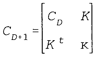


Claims

Priority Applications (4)
| Application Number | Priority Date | Filing Date | Title |
|---|---|---|---|
| EP99933675A EP1092196A1 (en) | 1998-07-02 | 1999-07-02 | An adaptive and reliable system and method for operations management |
| JP2000558464A JP2002520695A (en) | 1998-07-02 | 1999-07-02 | System and method for adaptive and reliable operation management |
| CA002336368A CA2336368A1 (en) | 1998-07-02 | 1999-07-02 | An adaptive and reliable system and method for operations management |
| AU49677/99A AU4967799A (en) | 1998-07-02 | 1999-07-02 | An adaptive and reliable system and method for operations management |
Applications Claiming Priority (4)
| Application Number | Priority Date | Filing Date | Title |
|---|---|---|---|
| US9165698P | 1998-07-02 | 1998-07-02 | |
| US60/091,656 | 1998-07-02 | ||
| US9175398P | 1998-07-06 | 1998-07-06 | |
| US60/091,753 | 1998-07-06 |
Publications (2)
| Publication Number | Publication Date |
|---|---|
| WO2000002136A1 true WO2000002136A1 (en) | 2000-01-13 |
| WO2000002136A9 WO2000002136A9 (en) | 2000-10-26 |
Family
ID=26784200
Family Applications (1)
| Application Number | Title | Priority Date | Filing Date |
|---|---|---|---|
| PCT/US1999/015096 WO2000002136A1 (en) | 1998-07-02 | 1999-07-02 | An adaptive and reliable system and method for operations management |
Country Status (5)
| Country | Link |
|---|---|
| EP (1) | EP1092196A1 (en) |
| JP (1) | JP2002520695A (en) |
| AU (1) | AU4967799A (en) |
| CA (1) | CA2336368A1 (en) |
| WO (1) | WO2000002136A1 (en) |
Cited By (12)
| Publication number | Priority date | Publication date | Assignee | Title |
|---|---|---|---|---|
| US6317725B1 (en) * | 1998-02-16 | 2001-11-13 | Nec Corporation | Production management system |
| JP2002269321A (en) * | 2001-03-14 | 2002-09-20 | Fujitsu Ltd | System and program for analyzing commercial transaction |
| US6952678B2 (en) | 2000-09-01 | 2005-10-04 | Askme Corporation | Method, apparatus, and manufacture for facilitating a self-organizing workforce |
| US7333960B2 (en) | 2003-08-01 | 2008-02-19 | Icosystem Corporation | Methods and systems for applying genetic operators to determine system conditions |
| US7356518B2 (en) | 2003-08-27 | 2008-04-08 | Icosystem Corporation | Methods and systems for multi-participant interactive evolutionary computing |
| US7444309B2 (en) | 2001-10-31 | 2008-10-28 | Icosystem Corporation | Method and system for implementing evolutionary algorithms |
| JP2009070406A (en) * | 2008-11-28 | 2009-04-02 | Ricoh Co Ltd | Display method, program, and recording medium |
| AU2010246536B2 (en) * | 2010-11-30 | 2014-01-23 | Finsuite Pty Ltd | Schematic Corporate Device and System |
| WO2015073036A1 (en) * | 2013-11-15 | 2015-05-21 | Hewlett-Packard Development Company, L.P. | Selectng a task or a solution |
| US9645573B2 (en) | 2014-11-25 | 2017-05-09 | International Business Machines Corporation | Reliability monitor test strategy definition |
| US10755225B2 (en) | 2014-08-06 | 2020-08-25 | United Parcel Service Of America, Inc. | Concepts for monitoring shipments |
| US10776745B2 (en) | 2014-08-06 | 2020-09-15 | United Parcel Service Of America, Inc. | Concepts for monitoring shipments |
Families Citing this family (3)
| Publication number | Priority date | Publication date | Assignee | Title |
|---|---|---|---|---|
| JP2007122154A (en) * | 2005-10-25 | 2007-05-17 | Kozo Nagata | Solution system and solution method for supply chain |
| US20210158259A1 (en) * | 2019-11-25 | 2021-05-27 | David Michael Evans | Orchestrated intelligent supply chain optimizer |
| CN111507007B (en) * | 2020-04-22 | 2023-07-07 | 西安工业大学 | Method for constructing general structure of three-dimensional assembly model based on conjugate subgraph |
Citations (7)
| Publication number | Priority date | Publication date | Assignee | Title |
|---|---|---|---|---|
| US5541848A (en) * | 1994-12-15 | 1996-07-30 | Atlantic Richfield Company | Genetic method of scheduling the delivery of non-uniform inventory |
| US5687292A (en) * | 1994-06-13 | 1997-11-11 | Telefonaktiebolaget Lm Ericsson | Device and method for determining a distribution of resources of a physical network |
| US5704012A (en) * | 1993-10-08 | 1997-12-30 | International Business Machines Corporation | Adaptive resource allocation using neural networks |
| US5761381A (en) * | 1995-08-31 | 1998-06-02 | International Computers Limited | Computer system using genetic optimization techniques |
| US5835901A (en) * | 1994-01-25 | 1998-11-10 | Martin Marietta Corporation | Perceptive system including a neural network |
| US5864633A (en) * | 1996-05-17 | 1999-01-26 | Therma-Wave, Inc. | Method and apparatus for optical data analysis |
| US5897629A (en) * | 1996-05-29 | 1999-04-27 | Fujitsu Limited | Apparatus for solving optimization problems and delivery planning system |
-
1999
- 1999-07-02 JP JP2000558464A patent/JP2002520695A/en not_active Abandoned
- 1999-07-02 WO PCT/US1999/015096 patent/WO2000002136A1/en not_active Application Discontinuation
- 1999-07-02 AU AU49677/99A patent/AU4967799A/en not_active Abandoned
- 1999-07-02 EP EP99933675A patent/EP1092196A1/en not_active Withdrawn
- 1999-07-02 CA CA002336368A patent/CA2336368A1/en not_active Abandoned
Patent Citations (7)
| Publication number | Priority date | Publication date | Assignee | Title |
|---|---|---|---|---|
| US5704012A (en) * | 1993-10-08 | 1997-12-30 | International Business Machines Corporation | Adaptive resource allocation using neural networks |
| US5835901A (en) * | 1994-01-25 | 1998-11-10 | Martin Marietta Corporation | Perceptive system including a neural network |
| US5687292A (en) * | 1994-06-13 | 1997-11-11 | Telefonaktiebolaget Lm Ericsson | Device and method for determining a distribution of resources of a physical network |
| US5541848A (en) * | 1994-12-15 | 1996-07-30 | Atlantic Richfield Company | Genetic method of scheduling the delivery of non-uniform inventory |
| US5761381A (en) * | 1995-08-31 | 1998-06-02 | International Computers Limited | Computer system using genetic optimization techniques |
| US5864633A (en) * | 1996-05-17 | 1999-01-26 | Therma-Wave, Inc. | Method and apparatus for optical data analysis |
| US5897629A (en) * | 1996-05-29 | 1999-04-27 | Fujitsu Limited | Apparatus for solving optimization problems and delivery planning system |
Cited By (13)
| Publication number | Priority date | Publication date | Assignee | Title |
|---|---|---|---|---|
| US6317725B1 (en) * | 1998-02-16 | 2001-11-13 | Nec Corporation | Production management system |
| US6952678B2 (en) | 2000-09-01 | 2005-10-04 | Askme Corporation | Method, apparatus, and manufacture for facilitating a self-organizing workforce |
| JP2002269321A (en) * | 2001-03-14 | 2002-09-20 | Fujitsu Ltd | System and program for analyzing commercial transaction |
| US7444309B2 (en) | 2001-10-31 | 2008-10-28 | Icosystem Corporation | Method and system for implementing evolutionary algorithms |
| US7333960B2 (en) | 2003-08-01 | 2008-02-19 | Icosystem Corporation | Methods and systems for applying genetic operators to determine system conditions |
| US7356518B2 (en) | 2003-08-27 | 2008-04-08 | Icosystem Corporation | Methods and systems for multi-participant interactive evolutionary computing |
| JP2009070406A (en) * | 2008-11-28 | 2009-04-02 | Ricoh Co Ltd | Display method, program, and recording medium |
| AU2010246536B2 (en) * | 2010-11-30 | 2014-01-23 | Finsuite Pty Ltd | Schematic Corporate Device and System |
| WO2015073036A1 (en) * | 2013-11-15 | 2015-05-21 | Hewlett-Packard Development Company, L.P. | Selectng a task or a solution |
| US10755225B2 (en) | 2014-08-06 | 2020-08-25 | United Parcel Service Of America, Inc. | Concepts for monitoring shipments |
| US10776745B2 (en) | 2014-08-06 | 2020-09-15 | United Parcel Service Of America, Inc. | Concepts for monitoring shipments |
| US11783276B2 (en) | 2014-08-06 | 2023-10-10 | United Parcel Service Of America, Inc. | Concepts for monitoring shipments |
| US9645573B2 (en) | 2014-11-25 | 2017-05-09 | International Business Machines Corporation | Reliability monitor test strategy definition |
Also Published As
| Publication number | Publication date |
|---|---|
| JP2002520695A (en) | 2002-07-09 |
| CA2336368A1 (en) | 2000-01-13 |
| AU4967799A (en) | 2000-01-24 |
| WO2000002136A9 (en) | 2000-10-26 |
| EP1092196A1 (en) | 2001-04-18 |
Similar Documents
| Publication | Publication Date | Title |
|---|---|---|
| US20030014379A1 (en) | Adaptive and reliable system and method for operations management | |
| US7752064B2 (en) | System and method for infrastructure design | |
| Venugopal et al. | Neural Networks and Statistical Techniques in Marketing Research: AConceptual Comparison | |
| Simchi-Levi et al. | Handbook of quantitative supply chain analysis: modeling in the e-business era | |
| WO2000002136A1 (en) | An adaptive and reliable system and method for operations management | |
| US20050149381A1 (en) | Method and system for estimating price elasticity of product demand | |
| US20180299540A1 (en) | Method, apparatus and system for location detection and object aggregation | |
| CA2519693A1 (en) | Performing predictive pricing based on historical data | |
| Meharie et al. | An effective approach to input variable selection for preliminary cost estimation of construction projects | |
| Murugappan et al. | Performance analysis of clustering methods for balanced multi-robot task allocations | |
| Scherer et al. | On the practical art of state definitions for Markov decision process construction | |
| KR102223844B1 (en) | Method for providing mentoring service connected investment, system and computer-readable medium recording the method | |
| Hsu et al. | A back-propagation neural network with a distributed lag model for semiconductor vendor-managed inventory | |
| Silva et al. | Deep reinforcement learning for stochastic last-mile delivery with crowdshipping | |
| Hong et al. | Probabilistic reliable linguistic term sets applied to investment project selection with the gained and lost dominance score method | |
| Fernandez et al. | An interval-based evolutionary approach to portfolio optimization of new product development projects | |
| Baykasoglu et al. | Contractor selection with multi criteria decision support tools | |
| Soroor et al. | An advanced adoption model and an algorithm of evaluation agents in automated supplier ranking | |
| Liu et al. | Product and ancillary pricing optimization: Market share analytics via perturbed utility model | |
| Afshar et al. | An automated deep reinforcement learning pipeline for dynamic pricing | |
| Li et al. | BCVR: A methodological framework for industrial performance management and decision-support | |
| Alamdari et al. | Deep reinforcement learning in seat inventory control problem: an action generation approach | |
| Wang et al. | Replenishment and delivery optimization for unmanned vending machines service system based on fuzzy clustering | |
| Eydi et al. | A multi-period multiple objective uncertain programming model to allocate order for supplier selection problem | |
| Zeydan et al. | A TOPSIS-based improved weighting approach with evolutionary computation |
Legal Events
| Date | Code | Title | Description |
|---|---|---|---|
| AK | Designated states |
Kind code of ref document: A1 Designated state(s): AE AL AM AT AU AZ BA BB BG BR BY CA CH CN CU CZ DE DK EE ES FI GB GD GE GH GM HR HU ID IL IN IS JP KE KG KP KR KZ LC LK LR LS LT LU LV MD MG MK MN MW MX NO NZ PL PT RO RU SD SE SG SI SK SL TJ TM TR TT UA UG UZ VN YU ZA ZW |
|
| AL | Designated countries for regional patents |
Kind code of ref document: A1 Designated state(s): GH GM KE LS MW SD SL SZ UG ZW AM AZ BY KG KZ MD RU TJ TM AT BE CH CY DE DK ES FI FR GB GR IE IT LU MC NL PT SE BF BJ CF CG CI CM GA GN GW ML MR NE SN TD TG |
|
| 121 | Ep: the epo has been informed by wipo that ep was designated in this application | ||
| DFPE | Request for preliminary examination filed prior to expiration of 19th month from priority date (pct application filed before 20040101) | ||
| AK | Designated states |
Kind code of ref document: C2 Designated state(s): AE AL AM AT AU AZ BA BB BG BR BY CA CH CN CU CZ DE DK EE ES FI GB GD GE GH GM HR HU ID IL IN IS JP KE KG KP KR KZ LC LK LR LS LT LU LV MD MG MK MN MW MX NO NZ PL PT RO RU SD SE SG SI SK SL TJ TM TR TT UA UG UZ VN YU ZA ZW |
|
| AL | Designated countries for regional patents |
Kind code of ref document: C2 Designated state(s): GH GM KE LS MW SD SL SZ UG ZW AM AZ BY KG KZ MD RU TJ TM AT BE CH CY DE DK ES FI FR GB GR IE IT LU MC NL PT SE BF BJ CF CG CI CM GA GN GW ML MR NE SN TD TG |
|
| COP | Corrected version of pamphlet |
Free format text: PAGES 1/33-33/33, DRAWINGS, REPLACED BY NEW PAGES 1/30-30/30; DUE TO LATE TRANSMITTAL BY THE RECEIVING OFFICE |
|
| ENP | Entry into the national phase |
Ref document number: 2336368 Country of ref document: CA |
|
| ENP | Entry into the national phase |
Ref country code: JP Ref document number: 2000 558464 Kind code of ref document: A Format of ref document f/p: F |
|
| WWE | Wipo information: entry into national phase |
Ref document number: 1999933675 Country of ref document: EP |
|
| WWP | Wipo information: published in national office |
Ref document number: 1999933675 Country of ref document: EP |
|
| REG | Reference to national code |
Ref country code: DE Ref legal event code: 8642 |
|
| WWW | Wipo information: withdrawn in national office |
Ref document number: 1999933675 Country of ref document: EP |