US8784327B2 - Method and system for obtaining dimension related information for a flow channel - Google Patents
Method and system for obtaining dimension related information for a flow channel Download PDFInfo
- Publication number
- US8784327B2 US8784327B2 US12/372,565 US37256509A US8784327B2 US 8784327 B2 US8784327 B2 US 8784327B2 US 37256509 A US37256509 A US 37256509A US 8784327 B2 US8784327 B2 US 8784327B2
- Authority
- US
- United States
- Prior art keywords
- velocity
- channel
- flow
- fluid
- dimensionless
- Prior art date
- Legal status (The legal status is an assumption and is not a legal conclusion. Google has not performed a legal analysis and makes no representation as to the accuracy of the status listed.)
- Active, expires
Links
Images

Classifications
-
- A—HUMAN NECESSITIES
- A61—MEDICAL OR VETERINARY SCIENCE; HYGIENE
- A61B—DIAGNOSIS; SURGERY; IDENTIFICATION
- A61B5/00—Measuring for diagnostic purposes; Identification of persons
- A61B5/02—Detecting, measuring or recording pulse, heart rate, blood pressure or blood flow; Combined pulse/heart-rate/blood pressure determination; Evaluating a cardiovascular condition not otherwise provided for, e.g. using combinations of techniques provided for in this group with electrocardiography or electroauscultation; Heart catheters for measuring blood pressure
- A61B5/026—Measuring blood flow
-
- A—HUMAN NECESSITIES
- A61—MEDICAL OR VETERINARY SCIENCE; HYGIENE
- A61B—DIAGNOSIS; SURGERY; IDENTIFICATION
- A61B5/00—Measuring for diagnostic purposes; Identification of persons
- A61B5/02—Detecting, measuring or recording pulse, heart rate, blood pressure or blood flow; Combined pulse/heart-rate/blood pressure determination; Evaluating a cardiovascular condition not otherwise provided for, e.g. using combinations of techniques provided for in this group with electrocardiography or electroauscultation; Heart catheters for measuring blood pressure
- A61B5/02007—Evaluating blood vessel condition, e.g. elasticity, compliance
-
- A—HUMAN NECESSITIES
- A61—MEDICAL OR VETERINARY SCIENCE; HYGIENE
- A61B—DIAGNOSIS; SURGERY; IDENTIFICATION
- A61B5/00—Measuring for diagnostic purposes; Identification of persons
- A61B5/72—Signal processing specially adapted for physiological signals or for diagnostic purposes
-
- A—HUMAN NECESSITIES
- A61—MEDICAL OR VETERINARY SCIENCE; HYGIENE
- A61B—DIAGNOSIS; SURGERY; IDENTIFICATION
- A61B8/00—Diagnosis using ultrasonic, sonic or infrasonic waves
- A61B8/06—Measuring blood flow
Definitions
- the present invention relates to a method and system for determining channel dimension related information based on measurements performed on a fluid flowing through a channel of unknown dimensions.
- the invention allows for using a non-invasive interrogating signal to obtain substantially real-time velocity measurements and, in turn, to use such measurements to assess properties of the channel containing the fluid, including instantaneous volumetric flow rate.
- dimension related information for a flow channel where it is difficult or undesirable to access the flow channel or otherwise obtain a direct dimensional measurement.
- Obtaining such information is particularly challenging where channel dimensions vary over time.
- An example is obtaining dimension related information for a blood vessel (i.e., artery or vein), such as the ascending aorta, of a human or other patient.
- the dimension related information of interest may be a dimension of the flow channel or other information derived from or dependent on dimension such as quantitative flow rate information (e.g., volumetric or mass flow rate), vessel elasticity/health, volumetric delivery per heartbeat, ejection fraction or the like.
- VFR volumetric flow rate
- the volumetric flow rate (“VFR”) of a fluid flowing through a channel is dependent on the velocity of the fluid and the cross-sectional area of the channel.
- Instantaneous VFRs may be calculated when these values are known between short time intervals that may be considered instantaneous. Determining the VFR of fluids in patients is useful, for example, in assessing cardiac performance.
- the fluid is a liquid, e.g., blood, that is flowing through a closed channel, such as the aorta.
- a closed channel such as the aorta.
- time-varying markers such as a dye, chilled normal saline, or blood warmed with a small electric heater
- the rate of change of the marker is then used to estimate the overall flow rate of blood.
- the catheter is most commonly introduced into the patient's femoral artery and threaded through the venous system into and through the heart to the pulmonary artery.
- a variant of this method introduces a dye without a catheter, but requires an injection near the atrium and measures the dye concentration at a point such as the ear.
- these time-varying marker methods rely on the marker dilution transient and provide bulk flow data, rather than flow rate data through a channel.
- the time-varying marker methods do not provide instantaneous VFRs.
- Fick methods calculate cardiac output using the difference in oxygen content between the arterial and mixed venous blood and the total body oxygen consumption.
- the classic Fick method uses arterial and pulmonary artery catheters to measure the oxygen content.
- Related methods measure oxygen and carbon dioxide data in a patient's airways to avoid using catheters.
- Fick methods measure bulk cardiac output, and not flow rates.
- other methods such as bioimpedance, may also be used to measure cardiac output.
- these methods do not measure flow rate, but rather only cardiac output.
- Conventional flow channel measurements may also be problematic, uncertain or inaccurate due to measurement artifact and associated processing.
- ultrasound measurements of an ascending aorta are problematic due to the difficulty of isolating the signal of interest from measurement artifact.
- Such artifact may relate to echoes from physiological material outside of the aorta or other channel that tend to obscure the signal of interest, in-channel noise sources and other interfering components.
- Some approaches have attempted to minimize certain artifact components by disposing the probe in close proximity to the aorta, thus incurring a morbidity trade-off.
- Other approaches attempt to minimize certain artifact components by employing a very narrow signal, but thereby complicate targeting of the aorta or other channel under consideration.
- a broad objective of the present invention is to provide a method and system for obtaining dimension related information for a flow channel, including a flow channel of a patient such as a blood vessel, based on qualitative flow rate information, e.g., velocity measurements.
- a related objective involves determining a quantitative flow rate such as a volumetric flow rate(s) (“VFR”) of a fluid flowing through a channel.
- VFR volumetric flow rate
- Another object of the present invention is to provide a method and system for non-invasive determination of a VFR of a fluid (e.g. blood) flowing through a living patient.
- a further related object is to provide a non-invasive method and system for determining fluid channel dimensions and combining the fluid channel dimension data with fluid velocity data to determine instantaneous VFR data.
- an object of the present invention is to use the same signals to measure fluid velocity data and determine fluid channel dimensions.
- a still further object of the present invention is to noninvasively obtain substantially real time velocity related and dimensional information for a flow channel such as a blood vessel, so as to enable instantaneous qualitative flow rate information, including for channels having dimensions that vary with time. It is also an object of the present invention to accurately account for artifacts associated with measurements related to a flow channel.
- Another object of the present invention is to provide for a rapid computation of otherwise computationally intractable formulae.
- the present invention allows for determining dimension related information for a flow channel without introducing a probe into the patient, thereby reducing pain and discomfort and reducing the likelihood of other problems such as the possibility of infection. Additionally, the present invention allows for obtaining such a measurement quickly, simply and at a reasonable cost.
- the present invention also enables measurements that can be used to determine instantaneous VFRs to enable clinicians to examine temporal changes and combine VFR measurements with other vital sign measurements, such as an electrocardiogram (EKG) measurement.
- EKG electrocardiogram
- flow characteristic information for a flow of a physiological material in a patient is used to obtain processed information related to a dimension of a flow channel.
- This aspect of the invention may be implemented as a process performed, at least in part, by a processor, and may be embodied, for example, in a software product or other logic, a processing unit for executing such logic, or a system for use in performing associated medical procedures.
- the flow characteristic information is qualitative flow characteristic information, i.e., information related to a flow velocity or derivatives thereof.
- flow velocity may be invasively or noninvasively measured at one or more points relative to a cross-section of a channel. Such flow velocity measurements may be used to calculate derivative information such as average flow velocity for that channel cross-section or information related to change in velocity relative to a channel dimension such as radius.
- the flow velocity measurements may also be used in calculating other parameters that characterize an instantaneous velocity profile. Such measurements may be repeated to provide derivative information related to a temporal change in velocity profile. It will thus be appreciated that the flow characteristic information may be provided in various forms, or be characterized by different parameters.
- the flow characteristic information may be based on a single or multiple measurements performed with respect to the flow channel under consideration. Additionally, such flow characteristic information may be used in multiple steps of a calculation, e.g., velocity profile information may be used to derive first processed information such as dimension related information, and the first processed information may be combined with average velocity or other flow characteristic information to derive second processed information.
- velocity profile information may be used to derive first processed information such as dimension related information, and the first processed information may be combined with average velocity or other flow characteristic information to derive second processed information.
- such information can vary depending on the particular inventive implementation under consideration.
- such information may be obtained in the form of an analog or digital signal, received either directly from a measurement device or via intervening processing.
- the flow characteristic information may be obtained by performing medical procedures on a patient.
- information such as flow velocity measurements may be obtained invasively, e.g., by introducing measurement elements into the flow channel or positioning a probe within the patient adjacent to the flow channel, or noninvasively, e.g., by receiving a signal from the channel such as an echo signal in the case of ultrasound modalities.
- the obtainment of such information can be synchronized with physiological processes of interest in accordance with the present invention.
- the processed information obtained using the flow characteristic information can vary depending on the application under consideration.
- Such information may include, for example, dimensional information regarding the flow channel such as a radius, major/minor axis dimension(s), cross-sectional area or other parameters characteristic of channel dimension; information derived from dimensional information such as a quantitative flow rate; or information otherwise dependent on such dimensional information (even if dimensional information is not determined as an intermediate step).
- dimensional information regarding the flow channel such as a radius, major/minor axis dimension(s), cross-sectional area or other parameters characteristic of channel dimension
- information derived from dimensional information such as a quantitative flow rate
- information otherwise dependent on such dimensional information even if dimensional information is not determined as an intermediate step.
- Examples of medical information that may be obtained in this regard include: the area, volumetric flow rate, pressure gradient, blood volume over time period of interest or elasticity of a blood vessel; and a cardiac pumping cycle period, volumetric delivery or ventricle ejection fraction of a patient.
- An application of particular interest relates to determining the volumetric flow rate of a fluid channel such as an ascending aorta of a patient.
- the present inventor has recognized that temporal changes in a moving fluid's velocity profile can be analyzed to calculate dimensions of a fluid channel.
- the fluid channel dimensions and the fluid velocity profile data can be combined to calculate a VFR for the fluid flowing in the channel.
- unsteady laminar flow along the length of a channel contains fluid elements moving at velocities that depend upon their distance from the channel walls, the channel geometry, the pressure gradient acting on the fluid, the fluid properties, and the initial velocities of the fluid elements.
- the velocities of fluid elements away from the channel walls regularly transition to velocities that depend upon the distance from the channel walls. When the pressure gradient does not reverse direction, the velocities of the fluid elements that are farthest from the walls are the greatest.
- the shape and dimensions of the pattern that these fluid velocities take in relation to the geometry of the channel defines a velocity profile.
- the geometry of the channel can be characterized using one or more dimensionless variables that relate dimensional values, such as a given point on the radius across a circular cross-section, to the largest extent of the dimension under consideration.
- the dimensionless radius can be defined as the radius at any point divided by the overall radius of the tube.
- One or more dimensionless variables can be used to characterize geometries, e.g. one dimensionless radius characterizes a circular tube and two dimensionless axes characterize an elliptical tube (one for the major axis and one for the minor axis). More complicated geometries can be represented by multivariate functions or the like.
- the time required for velocity profiles to change from one shape to another may be characterized by dimensionless time.
- a definition of dimensionless time involves the fluid's viscosity and density along with time and overall channel dimensions.
- a further aspect of the present invention is directed to a method for externally measuring a velocity of a fluid flowing through a channel.
- the method entails measuring the velocity of the fluid flowing through the channel using a non-invasive means such as an interrogating signal.
- the measured velocity is used to calculate an area of the channel, e.g. a cross-sectional area, which is then utilized along with the measured velocity to calculate at least one VFR for the fluid flowing through the channel.
- the velocity of the fluid may be measured using an ultrasonic interrogating signal. Such a velocity measurement may be characterized by a velocity profile.
- a velocity profile function may be used to calculate velocity profile parameters for the velocity profile at a first time. The velocity profile parameters may then be utilized to calculate a mean velocity of the fluid flowing through the channel.
- a dimensionless time may be calculated using the velocity profile parameters and a functional relationship characterizing how velocity profiles change with time.
- the dimensionless time is related to the dimensions of the channel such that the dimensions of the channel may be calculated and used to determine a cross-sectional area of the channel.
- the cross-sectional area of the channel may be utilized with the mean fluid velocity to determine at least one VFR for the fluid flowing through the channel.
- errors in the velocity measurement may be accounted for by distinguishing between signals emanating from the moving fluid and signals emanating from surrounding regions that may produce signal noise that would otherwise confound determining the correct velocity profile and fluid channel dimensions. Further in this regard, random measurement errors may be absorbed such that the errors can be discriminated from the actual velocity profile.
- a system for calculating VFRs includes a data processor that uses a measured fluid velocity to calculate an area of a channel and uses the area of the channel and the measured fluid velocity to calculate at least one VFR for the fluid flowing through the channel.
- the system may further include one or more output modules to provide an output to a user indicative of at least one volumetric flow rate.
- the system may further include a velocity measuring device to measure the fluid velocity and provide the measured velocity to the data processor.
- the data processor may include logic for calculating channel dimensions using two or more flow velocity profiles or velocity flow distributions, and logic for using channel dimension data in conjunction with measured velocity data to calculate at least one VFR.
- Such a system can also include logic for discriminating the flow velocity distribution from measured data that also includes data other than that associated with the material flowing in a channel.
- Such a system can also include logic for calculating pressure gradients and other derived parameters such as the rate of change of VFR's or measures of channel elasticity that relate channel dimensions and pressure gradients.
- the data processor will typically be one or more electronic devices that use one or more semiconductor components such as microprocessors, microcontrollers, or memory elements.
- the data processor will typically have a data storage element, employing non-volatile memory means, such as one or more magnetic media (such as disk drives), optical media (such as CD ROM), or semiconductor means (such as EPROM or EEPROM).
- the data storage element could be used, for example, to store data used to facilitate computations. Examples of data that may be stored to facilitate computations include without limitation, data stored for avoiding or reducing the need to calculate special functions, such as Bessel, Lommel, Bessell-zero, modified Bessel, Gamma, log-Gamma, and hypergeometric functions.
- the velocity measurement device may use an interrogating signal that is transmitted into the region containing the channel with the flowing fluid for which the VFR or other parameters are to be determined.
- an interrogating signal may use transmitted energy that has amplitudes that vary with time, such as ultrasonic energy or electromagnetic energy (including light that is in the visible spectrum as well as electromagnetic radiation that has frequencies below or above the visible spectrum).
- Ultrasonic energy will typically use frequencies in the range between 50 kHz and 50 MHz and more typically in the range between 500 kHz and 5 MHz.
- Such interrogating signals may be sent either continuously or in pulses.
- the velocity measurement device can use changes in velocity or phase that occur when the interrogating signal interacts with moving material that either backscatters energy or produces echoes.
- Doppler measurements includes without limitation, Doppler measurements.
- a system for calculating VFRs may further include logic for timing measurements based on external signals.
- external timing signals include those related to flow inducing phenomena such as signals related to factors that cause pressure gradient changes.
- the system can use signals related to a heart's electrical activity, such as electrocardiograph (EKG) signals, to sequence or control when measurements are made or to correlate measurements. In this regard, controlling when measurements are made can influence when interrogation signals are transmitted and correlating measurements can influence how measurements that have been made are interpreted.
- EKG electrocardiograph
- the one or more data output modules may be of any suitable type such as displays, audible sound producing elements, or data output ports such as those that transmit electronic or electromagnetic signals and associated local or wide-area network ports.
- the system may also include one or more controls such as power controls, signal sensitivity adjustments, or adjustments that cause signals or calculated results to be altered based on the characteristics of the flowing medium.
- Such adjustments may include those that are based on fluid properties and include adjustments for standard fluid properties. Some examples of such standard fluid properties include without limitation, viscosity, density, and kinematic viscosity.
- Adjustments based on fluid property can include properties correlated with standard fluid properties and include hematocrit as a correlated fluid property. Adjustments based on hematocrit can include using single values of hematocrit, ranges of hematocrit, or patient-specific data that are related to hematocrit such as patient species, age, or sex.
- a software product for calculating dimension related information for a fluid channel includes data processor instructions that are executed on a processor, e.g. a data processor, to use a measured flow characteristic such as information related to fluid velocity to calculate dimension related information, such as a channel radius or area for a channel.
- the software product may further include instructions for using dimension related information together with the measured flow characteristic to calculate at least one additional value, which may be a further dimension related value such as a VFR for the fluid flowing through the channel.
- the software product may further include output instructions configured to provide an output to a user indicative of at least one of the flow characteristic, the dimension related information and the additional value.
- the software product may further include velocity measuring instructions for obtaining a measurement of the fluid velocity and providing the measured velocity to the data processor.
- the data processor instructions may be configured to calculate channel dimensions using two or more flow velocity profiles or velocity flow distributions, and instructions for using channel dimension data in conjunction with measured velocity data to calculate at least one VFR.
- such a software product may also include instructions for discriminating the flow velocity distribution from measured data that also includes data other than that associated with the material flowing in a channel.
- Such a software product can also include instructions for calculating pressure gradients and other derived parameters such as the rate of change of VFR's or measures of channel elasticity that relate channel dimensions and pressure gradients.
- a software product for calculating VFRs may further include instructions for timing measurements based on external signals.
- external timing signals may include those related to flow inducing phenomena such as signals related to factors that cause pressure gradient changes.
- the software product could use signals related to a heart's electrical activity, such as electrocardiograph (EKG) signals, to sequence or control when measurements are made or to correlate measurements.
- EKG electrocardiograph
- substantially real-time velocity measurements and substantially real-time dimension related information are obtained for a patient flow channel at substantially the same time.
- the information may be obtained noninvasively such as by ultrasound processes based on the same or multiple signal sets.
- ultrasound measurements may be used, as discussed above, to obtain velocity profile information at successive times and information related to the temporal change in velocity profile may be used to derive dimension related information.
- additional dimension related information such as a VFR value or other derived information may be obtained.
- the successive velocity profile measurements may be made sufficiently close in time that other flow parameters such as channel cross-section and pressure gradient, may safely be assumed unchanged, or successive measurements may be pulse cycle synchronized and/or variations in other flow parameters may be taken into account.
- instantaneous results can be obtained, allowing for more timely presentation to physicians and improved correlation to physiological processes as may be desired.
- a method and apparatus are provided to account for artifacts in a signal used to determine information regarding a physiological material in motion, for example, a physiological fluid in a flow channel of a patient.
- the present inventor has recognized that such artifacts may relate to signal portions associated with surrounding material or noise associated with signal portions emanating from the flow channel.
- Some prior attempts to address artifacts have recognized, for example, that a spectral analysis of ultrasound information related to a flow channel exhibits bimodal characteristics but have assumed that frequency filtering can be employed to isolate a spectral portion of interest without introducing unacceptable inaccuracies.
- a mathematical model is provided that characterizes the input signal as a signal portion of interest and an undesired signal component.
- An analysis is then employed using the mathematical structure to mathematically absorb the undesired signal portion free from frequency filtering and the associated assumptions.
- multi-parameter functions may be used to parameterize the input signal including the undesired signal portion and well-founded statistical processes can be used to absorb the undesired components.
- well-founded statistical processes can be used to absorb the undesired components.
- in-channel and out-of-channel artifact can be absorbed.
- standard ultrasound measurements or more advanced measurements as disclosed herein may be accurately performed without positioning the probe within the patient adjacent to the channel, or without targeting complications associated with very narrow signals.
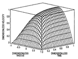
- FIG. 1 illustrates the dimensionless velocity profile for fully developed laminar flow
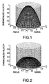
- FIG. 2 illustrates dimensionless velocity profile for developing laminar flow
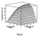
- FIG. 3 illustrates changes in velocity profiles after startup from zero velocity
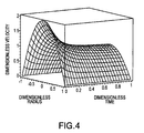
- FIG. 4 illustrates changes in velocity profiles after startup from non-zero velocity larger than that which will occur at steady state
- FIG. 5 illustrates changes in velocity profiles when the pressure gradient reverses direction
- FIG. 6 illustrates an interrogating signal and the regions producing measured signal
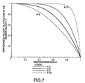
- FIG. 7 illustrates example dimensionless velocity profiles
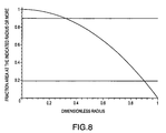
- FIG. 8 graphs the cumulative probability distribution of the area of a circle
- FIG. 9 illustrates how dimensionless velocity ( ⁇ ) changes with the fraction of cross-sectional area
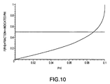
- FIG. 10 graphs an example cumulative probability function for dimensionless velocity for developing laminar flow
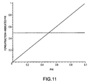
- FIG. 11 graphs an example cumulative probability function for dimensionless velocity for fully developed laminar flow
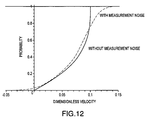
- FIG. 12 graphs example cumulative probability functions without noise and with noise
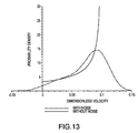
- FIG. 13 graphs example probability density functions without noise and with noise
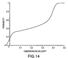
- FIG. 14 graphs an example cumulative probability function that includes a slow moving region and noise
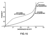
- FIG. 15 graphs example cumulative functions with and without sources of error
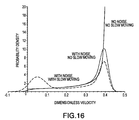
- FIG. 16 graphs example density functions with and without sources of error
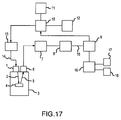
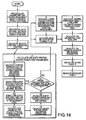
- FIG. 17 illustrates a block diagram of one embodiment of a system
- FIG. 18 illustrates one embodiment of the calculation sequence
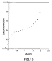
- FIG. 19 illustrates an example of spectral cumulative data points
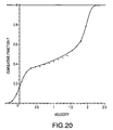
- FIG. 20 illustrates an example of spectral cumulative data point fitting in progress.
- unsteady laminar flow along the length of a channel contains fluid elements moving at velocities that depend upon their distance from the channel's walls, the channel's geometry, the pressure gradient acting on the fluid, the fluid's properties, and the initial velocities of the fluid elements.
- the velocities of fluid elements away from the channel's walls regularly transition to velocities that depend upon the distance from the channel's walls.
- the pressure gradient does not reverse direction the velocity of the fluid elements in that are farthest from the walls move the fastest.
- FIG. 1 illustrates the velocities for the case where the channel is a cylindrical tube and the pressure gradient has been applied long enough for the fluid flow to have reached steady state.
- the shape and dimensions of the pattern that the velocities of the fluid elements take in relation to the geometry of the channel is the velocity profile.
- the geometry of the channel can be characterized using dimensionless variables that relate dimension values, such as a value of a particular position relative to the radius across a circular cross-section, to the largest extent of the dimension under consideration.
- the dimensionless radius may be defined as the radius at any point divided by the overall radius of the tube.
- One or more dimensionless variables can be used to characterize geometries: one dimensionless radius characterizes a circular tube and two dimensionless axes characterize an elliptical tube (one for the major axis and one for the minor axis).
- proxies for a dimensionless variable may be used, such as aspect ratio wherein the aspect ratio is the ratio of major axis to minor axis in an ellipse, and which may be used in conjunction with the major dimensionless axis.
- dimensionless time The time required for velocity profiles to change from one shape to another may be characterized by dimensionless time.
- a definition of dimensionless time uses the fluid's viscosity and density along with time and overall channel dimensions.
- the general form of dimensionless time is
- ⁇ ⁇ ⁇ ⁇ t ⁇ ⁇ ⁇ f ⁇ ( D )
- ⁇ viscosity
- ⁇ density
- t time
- f(D) is a function of the parameters that characterize the channel's dimensions.
- f(D) has the dimensions of length-squared (L 2 ).
- Dimensionless time, ⁇ is also called a time constant and may be used to evaluate how many time constants are needed for a certain event to occur.
- blood flow in humans in the aorta follows a cyclic pattern determined by the heart rate.
- the heartbeat to heartbeat cycle lasts about 0.01 and 0.1 time constants (where the time constant utilized is described in greater detail below), and in most cases lasts between about 0.01 and 0.06 time constants.
- One aspect of the present invention is that it calculates VFRs for small and large time constants, including time constants at least as small as those encountered during cardiac heartbeat cycles in the aorta.
- the present invention uses changes between two or more velocity profiles that occur over one or more time intervals to calculate the value for dimensionless time and then uses the values of one or more instances of dimensionless time to calculate the parameters in f(D). Further in this regard, the present invention may use the parameters that characterize f(D) to calculate the cross-sectional area of the fluid channel. Still further in this regard, the present invention may use one or more calculated cross-sectional areas of the fluid channel in conjunction with one or more velocity profiles to calculate one or more VFRs.
- p 0 - p L L is the pressure gradient along the tube.
- Equations 1-3 define dimensionless variables for velocity, radius, and time respectively.
- equation 2 defines the dimensionless radius
- equation 3 defines the dimensionless time.
- Equation 3 can be solved for the radius, R:
- ⁇ ⁇ ( ⁇ ⁇ t ⁇ v z ) p 0 - p L L + ⁇ ⁇ ( ⁇ ⁇ r ⁇ r ⁇ ( ⁇ ⁇ r ⁇ v z ) ) r ( 5 )
- Equation 5 may then be multiplied by
- Equation 6 may be solved so that the following conditions are met:
- Reference 1 derives the following expression related to development of the velocity profile equation:
- J(n, x) is the n-th order Bessel function of the first kind and ⁇ (0,n) is the n-th positive real root of the zeroth order Bessel function of the first kind.
- the initial velocity distribution can be represented by a generalized equation.
- Various forms of such generalized equations may be used.
- Equation (12) may then be solved for B n by multiplying by J(0, ⁇ (0, m) ⁇ ) ⁇ and then integrating. The result is equation 13.
- the dimensionless time, ⁇ is a function of time.
- the velocity distribution starts developing from an initial velocity profile, which is characterized by equation (11) where a and k are the parameters that characterize the shape of the initial velocity distribution.
- EQ. 17 The result is EQ. 17:
- the flow profile depends upon four variables. Two of the variables, a and k, define the initial velocity profile. A third variable, ⁇ , characterizes the elapsed time. The fourth variable, ⁇ , characterizes the radius of the tube.
- the present invention uses data from velocity measurements to evaluate velocity profile parameters and then determines the values of other variables, such as channel dimensions based upon changes that occur in velocity profile parameters during a known time interval.
- the following method is an example of using changes in velocity profiles to determine channel dimensions and then to calculate VFRs and derived parameters.
- the general steps taken to calculate channel dimensions and VFRs using the above described formulas are as follows:
- equation (11) is an example of a function that characterizes velocity profiles.
- equation (11) is an example of a function that characterizes velocity profiles.
- such calculations may use only two data points or the calculations may use more than two data points in conjunction with statistical curve fitting techniques such as least squares or least absolute value methods.
- t (measured in, for example, seconds)
- t time interval
- k time interval
- the velocity profile change can be analyzed over a time period that is sufficiently short that changes in flow parameters such as channel dimension and pressure gradient can be safely assumed to be negligible.
- Such parameters vary with the patient's pulse cycle which will generally have a frequency between 0.5-4.0 Hz.
- the time interval within which changes in velocity profile parameters are analyzed is preferably no longer than about 0.025 seconds and, more preferably, no more than about 0.01 seconds. It will be appreciated, however, that the time interval(s) may alternatively be phase synchronized relative to the patient's pulse cycle or changes in flow parameters may be taken into account.
- equation (5) use an equation that relates dimensionless time to channel dimensions to calculate the channel's dimensions. For example, use equation (4), along with the known the values for t, viscosity, and density (or the kinematic viscosity, which is the quotient of viscosity and density) to calculate the tube's radius, R.
- (6) use the now known channel dimensions to calculate the channel's cross-sectional area, A. For example, use the radius, R, to calculate the cross-sectional area.
- v mean k ⁇ ⁇ a 2 + k
- a is the maximum dimensioned velocity that occurs at the time of measurement.
- (10) calculate the radius and pressure gradient at two different times and divide the change in radius by the change in pressure gradient to calculate a channel elasticity.
- FIG. 4 depicts the situation where the velocity is decelerating because the pressure gradient is decreasing.
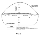
- FIG. 5 depicts the case where the pressure gradient has reversed directions.
- the dimensionless radius is on the axis labeled as r/R.
- FIG. 5 also illustrates a starting non-negative velocity profile at the bottom of the figure and a final steady state velocity profile at the top of the figure. Both of these profiles conform to the function form of equation (11).
- the curved middle velocity profile in FIG. 5 depicts a transitional velocity profile as the flow field reverses direction between the initial velocity profile and the final profile. The transition has the fluid in the center of the tube flowing down while the fluid at the edges has reversed and is flowing up. Such a case could occur, for example, if the aortic valve suffers significant backflow.
- a more complicated expression for the initial velocity profile is needed for cases where the pressure gradient reverses direction and will include more than the two parameters used in equation (11).
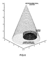
- FIG. 6 schematically portrays a case where an interrogating signal, such as ultrasound, is being beamed into a region containing a flowing fluid contained in a tube that is surrounded by a region of materials that are moving substantially more slowly (either in the same or opposite direction as the flowing fluid) than most of the material flowing in the tube.
- the slow moving material is essentially stationary compared to the flowing fluid.
- FIG. 6 only a portion of the tube containing fluid is shown in FIG. 6 .
- the situation portrayed in FIG. 6 is similar to that which would occur if an ultrasonic Doppler measurement were made of the blood flowing in the ascending aorta and the Doppler transducer is located in the suprasternal notch and aimed toward the heart.
- Some of the interrogating signal is echoed or backscattered, which is not depicted in FIG. 6 , and can be measured as a return signal.
- the frequency spectrum of the returned signal can be analyzed to produce estimates of the velocity profile of the region interrogated.
- a first source of error may be present in signals measured from the flowing region that add errors such as noise.
- a second source of error may be present from signals representing the slow moving material region that confound signals from the flowing region, so that slow moving velocity signals are added to the velocity signals from the flowing fluid.
- these two sources of errors are accounted for and prevented from producing significant errors in the estimated VFRs.
- the general solution is to absorb the errors by introducing mathematical structures that selectively pick these errors from the measured signal.
- the following is a derivation of a general and a specific example of error absorbing functions that may used to estimate distributions of measured signals or variables derived from measured signals.
- An example of a measured signal is the frequency from a Doppler measurement.
- Derived variables are variables calculated using one or more measured signals, such as velocities calculated from Doppler frequency measurements.
- ) the signal from the slow moving region, where
- ⁇ * maps to one and only one dimensionless velocity, ⁇ *.
- each dimensionless radius forms a circle around the center of the tube. All of the fluid moving through the tube at a particular ⁇ * will move with the same velocity ⁇ *.
- the probability of the fluid element being in a band extending from the outermost radius and inner radius is the ratio of the total cross-sectional area of the tube and the radius of the band of on the interval [ ⁇ ,1].
- Equation (21) can be interpreted as a cumulative probability distribution as illustrated in FIG. 8 .
- the maximum range of ⁇ is the interval [0,a].
- the variable a is the maximum value of the dimensionless velocity that occurred at the time that a velocity profile was measured.
- the fraction, F, in equation (22) can be interpreted as a probability and solved for the more traditional equation (23) representing the cumulative distribution of ⁇ that gives the fraction of the dimensionless velocities that are less than or equal to a particular ⁇ .
- the corresponding cumulative distribution has ⁇ defined between 0 and 1, as illustrated in FIG. 11 .
- ⁇ mean k ⁇ ⁇ a 2 + k ( 24 )
- v mean k ⁇ ⁇ a 2 + k ( 25 )
- Equation (23) is the cumulative probability function.
- Measurement errors alter the probability that the measured ⁇ is the correct value for ⁇ .
- the probability of having a particular ⁇ n occur and of having the noise added to it leading to a total value less than or equal to ⁇ is the product of the probability that will have ⁇ n times the probability that will have ⁇ n +noise ⁇ , which can be represented as p( ⁇ ) p( ⁇ n +noise ⁇ ).
- the product of these two probabilities is the cumulative probability that will have a total measured value ⁇ n ⁇ .
- the probability of having a particular ⁇ n is the product of the density function evaluated at ⁇ n d ⁇ .
- p( ⁇ n ) denote the probability of ⁇ taking on the specific value ⁇ n .
- the noise will have a distribution associated with it that is defined by a vector of parameters, H. For a Gaussian distribution, the parameters are the mean and standard deviation.
- the probability density function for the noise generating function be g noise ( ⁇ , H).
- the probability of having a particular ⁇ n and the noise centered around it being less than or equal to a velocity is the product of two probabilities: (probability of a particular ⁇ n ) ⁇ (probability of x+ ⁇ n ⁇ ) for a particular ⁇ n .
- the result is the joint probability given in equation (27):
- the cumulative probability is the probability that will have (x+ ⁇ n ⁇ ) for all ⁇ n is the sum of the individual probabilities for all ⁇ n , which is the same as integrating over all ⁇ n .
- the noise is a Gaussian (normal) distribution.
- the Central Limit Theorem states that the errors will have a Gaussian distribution about the true value. Therefore, the noise density function is centered about ⁇ n , and ⁇ n is the mean, and the noise function has a standard deviation ⁇ :
- g noise ⁇ ( ⁇ n ) 1 2 ⁇ 2 ⁇ e ( - 1 / 2 ⁇ ( x - ⁇ n ) 2 ⁇ 2 ) ⁇ ⁇ ⁇ ( 29 )
- p ⁇ ( ⁇ n , x + ⁇ n ⁇ ⁇ ) p ⁇ ( ⁇ n ) ⁇ ⁇ - ⁇ ⁇ ⁇ 1 2 ⁇ 2 ⁇ e ( - 1 / 2 ⁇ ( x - ⁇ n ) 2 ⁇ 2 ) ⁇ ⁇ ⁇ ⁇ ⁇ d x ( 30 )
- the cumulative probability is the probability that will have (x+ ⁇ n ⁇ ) for all ⁇ n is the sum of the individual probabilities for all ⁇ n , which is the same as integrating over all ⁇ n .
- FIG. 12 illustrates how Gaussian distributed random errors in the dimensionless velocity, ⁇ , affect the cumulative distribution. The errors spread the possible values for measured velocities so that they are both smaller and larger than the actual values that occur in the flowing fluid.
- Equation 28 is the general form of the cumulative spectral function with an error absorption function used to compensate for errors in the measured signal. Equation (32) is the specific case when the measurement error function is Gaussian. Other functional forms may be used instead of Gaussian, such as exponential, Cauchy, and Riceian.
- FIG. 13 illustrates how the probability density function is affected by the presence of Gaussian distributed random errors. It should be noted that the spreading of the probability density function, as exemplified in FIG. 13 , is caused by the measurement errors. Using error absorption functions to reduce or remove such errors, including those caused by random fluctuations that are commonly referred to as “noise”, is a general technique that is employed as part of the novel art of the current invention. It should be noted, however, that using error absorption functions to reduce or remove such errors according to the present method is particularly advantageous for determining velocity profiles (either dimensionless or with dimensions) and the subsequent calculations that lead to determining VFRs.
- the probability density functions are the spectral density functions that are produced by the frequency shifts produced by Doppler measurement methods.
- the parameters that characterize the error absorption function g noise ( ⁇ ,H) can be solved for, as well as for values of a and k that characterize the shape of the velocity profile. For example, if the noise absorption function is Gaussian then the value for standard deviation is solved for to characterize the noise absorption function.
- FIG. 9 illustrates an interrogating signal being used as part of a system to determine the velocity profile as part of the process of determining the VFR of the flowing region.
- the above error absorption functions can be used to reduce or remove measurement errors in the signals from the flowing region.
- the other source of possible error is the confounding signals that come from the slow flowing or non-flowing materials that are outside of the flowing region also shown in FIG. 9 .
- errors that may be caused by signals from slow moving and non-flowing materials may also be reducing or removed as follows.
- F flowing ( ⁇ ) represents the flowing material's distribution as expressed for example by equation 32, after it has been adjusted for the fraction of the region producing signals that have flow
- F slow ( ⁇ ) represents the material that is non-flowing (either not moving or slow moving).
- F slow ( ⁇ ) will be represented by a distribution for the non-flowing velocities, which is generally Gaussian, often with a non-zero mean. It should be noted, however, that the distribution most suitable for a particular application may include exponential, Cauchy, Riceian, or other distributions. Absent other information to the contrary, however, a Gaussian distribution is an appropriate distribution to use as the velocities of the non-flowing region are assumed to be moving much slower than those of the flowing regions. Additionally, the velocities of the non-flowing materials will be produced by a multitude of independent time-varying parameters that all invoke the Central Limit Theorem.
- a Gaussian distribution will be used as the error absorption function. It may be assumed that the slow moving velocities have a Gaussian distribution and that the mean may take on any value, including positive, negative, or zero at any instant when measurements are made. Additionally, the non-zero mean could occur, for example, if the measurement is of a region that includes the ascending aorta and the respiration processes occurring during the time of measurement causes a slow movement of the non-flowing region away from the location of the signal source. In this case, a fraction of the velocity signals will come from the flowing region and the balance will come from the slow moving region. The fraction of the signals from the two regions are used to weight the contributions from each region to the overall velocity distribution.
- the slow moving velocities produce Doppler echoes that are in addition to the echoes produced by the flowing velocities. They produce a total number of echoes at a particular velocity. In this regard, all of the echoes are added up and the total is used to normalize the number of counts at each velocity. In this regard, the number of counts from a particular region depend on its area, e.g. the number of counts that come from the slow moving region depend on its area, and the number of counts from the flow region depend on its area.
- the fractions of the total area for each region which is all that matters in the probability distribution, define how much weight is given to the signals from the flowing region and from the slow moving region.
- a s area for the slow moving region
- a f the area for the flow region
- the errors introduced by the slow moving region are characterized by two parameters.
- One parameter is the mean, ⁇ s , and the other is the standard deviation, ⁇ s .
- ⁇ s the mean
- ⁇ s the standard deviation
- ⁇ R the standard deviation
- FIG. 14 illustrates a cumulative probability function based on equation (35) for the case when the slow moving mean velocity is zero.
- Equation (35) The probability density function associated with equation (35) is given in equation (34):
- slow ⁇ ( ⁇ ) 1 2 ⁇ ( 1 - f f ) ⁇ 2 ⁇ e ( - 1 / 2 ⁇ ( ⁇ - ⁇ s ) 2 ⁇ s 2 ) ⁇ s ⁇ ⁇ + f f ⁇ ⁇ 0 a ⁇ ( 1 - x a ) ( 2 ⁇ 1 k - 1 ) ⁇ e ( - 1 / 2 ⁇ ( ⁇ - x ) 2 ⁇ 2 ) ⁇ 2 ⁇ ⁇ ⁇ ⁇ k ⁇ ⁇ a ⁇ ⁇ d x ( 36 )
- the preceding equations for the density functions and cumulative probability functions can also be used with dimensioned velocity instead of dimensionless velocity.
- the measured velocity data will have velocity units and are used where the variable ⁇ appears in the equations.
- velocity when either dimensioned velocity or dimensionless velocity may be used the general term “velocity” will be used.
- the measured data may be fit to one or more multi-parameter functions that include parameters for the velocity spectral density and for one or more error absorption functions. In another embodiment of the invention, the measured data may be fit to one or more multi-parameter functions that include parameters for the cumulative velocity spectrum and for one or more error absorption functions. Using the cumulative velocity spectrum instead of the density function reduces the effects of measurement errors because the cumulative spectrum is the smoothed integral of the density function.
- the fitting process will determine the values of the parameters that lead to the smallest errors between the measured data and the values predicted by the function.
- the smallest errors may be those determined using any suitable criteria and include minimizing the sum of least squared errors or minimizing the sum of least absolute value errors.
- the fitting process may fit all of the parameters as a set or it may first estimate values for the error absorption functions and remove the effects of errors before calculating values for the parameters that define the velocity spectra.
- the step-wise process of first removing the effects of errors leads to calculating approximately error-free data distributions.
- the error-free data are the velocity distribution for the material flowing in the channel for which the velocity spectra parameters are desired.
- the parameters are, for example, a and k calculated using equation (11) for use in equation (17) or equation (18) to calculate ⁇ , from which the radius R is calculated.
- an iterative process will generally be used during which values for the parameters are systematically adjusted to obtain the best fits to the velocity data.
- the iterative process systematically selects values for the error absorption parameters to calculate approximately error-free velocity distributions.
- the approximately error-free distributions are then used to calculate velocity distribution parameters.
- the velocity distribution parameters may be used to calculate revised values for the error absorption parameters.
- the revised error absorption parameters are then used to calculate a revised set of approximately error-free velocity distributions.
- the revised distribution is then used to recalculate values for the velocity distribution parameters.
- This iterative process of removing errors and calculating velocity distribution parameters is followed until a suitably good fit to the data occurs.
- Using this embodiment where errors are first removed from the measured data before the velocity distribution parameters are calculated has the advantage of generally producing better estimates of the velocity distribution parameters in a specified number of iterations. It should be noted that, obtaining accurate estimates of the velocity distribution parameters, such as the a and k in equation (18), is more important than calculating the values of other parameters because it is the velocity distribution parameters that are used to calculate dimensionless time, ⁇ , which then becomes the basis for calculating the flow channel's dimensions.
- the method described for reducing or eliminating errors using error absorption functions is ap plicable for use with both dimensionless velocity and dimensioned velocity.
- dimensioned velocity ⁇
- ⁇ dimensionless velocity
- the parameters associated with velocity have dimensions. For example, when a Gaussian distribution is used the mean and standard deviation will have velocity units.
- velocity profile parameters can have units, as for example, the variable a used above would have velocity units.
- equation (38) is the result of starting with equation (16) and solving for k t , assuming a known value, ⁇ i for selected values of ⁇ and ⁇ which can be denoted as ⁇ i and ⁇ i .
- equation (40) becomes equation (41), which can be solved iteratively for ⁇ when values for a, k, and k, are known.
- LommelS1 is the Lommel s function.
- one aspect of the present invention is precalculating the values for one or more terms in equations that implicitly define ⁇ in terms of the velocity profile characterization parameters and then using these precalculated values in a simplified equation that is used to develop an interpolating function that can be used to calculate the value for the time constant ⁇ .
- equation (41) can be used to precalculate values for its summation terms and these precalculated values used in a simplified equation to develop an interpolating function that relates k t to ⁇
- Equation (42) has the form of equation (43). Equation (39) and equations based on it, such as equation (41), can be converted into the form of equation (43).
- A will always be the same once ⁇ i has been selected.
- B and D will be constant for any selected ⁇ .
- the preferred method is to select values for ⁇ and k before measurements are needed and calculate and store values for B, C, D, and E ahead of time in a table.
- the values could be stored in a lookup table that is convenient for rapid access, such as if the entries are indexed by values of ⁇ and k.
- solving for ⁇ starts by selecting an assumed value for ⁇ and using the lookup table entries that bracket the actual value for k and the assumed value for ⁇ and calculate a value for k t using the actual value for a.
- a suitable interpolating function may be used, such as an interpolating polynomial, to relate ⁇ and k t .
- the interpolating function may then be used to solve for ⁇ using the actual value for k t .
- the derivation and description of the method for the efficient solution of ⁇ described above used ⁇ and dimensionless velocity.
- the same derivation and description of the method for efficient solution of ⁇ also applies using ⁇ and dimensioned velocity.
- the results using dimensioned velocity are identical except that the velocity profile parameter a includes velocity dimensions.
- Another aspect of the present invention is to identify the presence and nature of periodic and non-periodic flow rate behavior from one or more VFRs and the time intervals associated with the velocity profiles used to calculate the VFRs.
- the means used to identify the presence and nature of periodic flow rate behavior includes mathematical means such as Fourier analysis, artificial intelligence, statistical analysis, and non-linear analysis including those used in complexity theory and analysis. Identification of the presence and nature of the periodic flow rate behavior includes identifying changes in flow rate that reveal the cyclic behavior of flow, including the pumping cycle period from the heartbeat rate of living patients.
- Another aspect of the present invention is to use one or more VFRs in conjunction with one or more of the time intervals between velocity measurements to calculate the fluid volume that has flowed during the time elapsing between one or more time intervals.
- Such calculations are particularly advantageous when cyclic flows occur, such as when blood flows from a heart.
- Such calculations may be used to determine the blood volume delivered per cycle when the pumping cycle period is used in conjunction with data that relates fluid volume delivery with time.
- the heartbeat rate used to determine the volumetric delivery per heartbeat or other cycle may be an exogenous input such as a parameter entered by a user or data from an external source, such as an EKG, or it may be based on the identification of the presence and nature of the periodic and non-periodic flow rate behavior as described above. Volumetric delivery is a derived parameter.
- Another aspect of the present invention is to use volumetric delivery data per heartbeat in conjunction with total left ventricle volume to calculate ejection fraction.
- Total left ventricle volume may be estimated using means such as an interrogating signal that evaluates the nature or the signal returned from turbulent flow sections of a region energized by the interrogating signal.
- Ejection fraction is a derived parameter.
- the following description is related to a specific medical device application, although it will be appreciated that the present system is both useful for and readily employable in applications beyond the specific medical device application described.
- the present invention may take on configurations other than those described and illustrated.
- the means used for calculations may combine or separate functional units in configurations other than those described.
- the sequence of calculations may be done differently than those described.
- FIG. 17 illustrates a system that uses an ultrasonic transducer 1 to introduce an interrogating signal 2 into a patient 3 .
- the transducer may be any of various conventional ultrasound units and may provide the signal 2 in the form of a pulse train.
- the transducer 1 may be disposed external to the patient 3 , for example, in the suprasternal notch and may be directed so that the signal targets the ascending aorta. Depthwise targeting can be accomplished by processing return signal components received during the time window corresponding to the desired depth.
- the interrogating signal 2 backscatters from patient tissues 4 and a return signal 5 is detected by the receiving transducer 6 .
- the receiving transducer 6 converts the mechanical energy (not shown) of the return signal 5 into oscillating electrical signals (not shown) that are introduced into the analog amplification and processing module 7 .
- This module may perform a variety of functions including analog digital conversion, amplification, filtering and other signal enhancement.
- the output from the analog amplification and processing module 7 is a digitized stream of data that is the input to the digital processing module 8 .
- the digital processing module 8 converts the digitized signal data into frequency spectra, using known mathematical processes such as a fast fourier transform, and then into velocity data which becomes velocity vectors that the digital processing module 8 stores as vectors of digital dimensioned velocity profile data in a memory location (not shown) of the data processing module 9 .
- the data processing module 9 converts the velocity profile data (not shown) into a data vector (not shown) that represents a piecewise continuous dimensioned velocity spectral density function. Further processing of the density function data vector is described in more detail later.
- the digital processing module 8 may contain one or more microprocessors and one or more data storage means that enable it to make the calculations needed to determine VFRs and derived parameters.
- the data storage means contains values for parameters used in look-up tables that facilitate calculations that avoid or reduce the need to evaluate special functions. Additionally, certain values such as a channel dimension, average flow rate or the like may be predetermined and stored in cache or other storage for combination with values obtained in connection with a later measurement process.
- FIG. 17 also illustrates that the system has a control module 10 that receives setup parameters (not shown) from the user 11 .
- Setup parameters can include data such as patient parameters, e.g., hematocrit, and on/off signals regarding when data reading and processing should begin and end.
- the control module 10 receives signals from the data processing module 9 regarding the status of the received data (not shown) and changes in the interrogating signal 2 that are needed to improve or maintain quality measurement data.
- the control module 10 optionally receives signals of biological activity 12 , such as electrical signals related to cardiac activity.
- the biological signals 12 may be used to synchronize interrogating signals 2 to biological functions or to correlate calculated values such as VFRs to such biological functions.
- the control module 10 signals the transducer power module 13 when the interrogating signal 2 should begin and end.
- the transducer power module 13 provides the drive signal 14 to the ultrasonic transducer 1 .
- the data processing module 9 generates output data 15 that go to the output module 16 .
- the output module 16 generates visible displays 17 and audio devices 18 to inform the user of the system's operating status and the results of the system's interrogation of the patient 3 .
- the output module 16 may also include ports for providing data to other instruments (such as an EKG) or processing systems, for example, via a LAN or WAN.
- other instruments such as an EKG
- processing systems for example, via a LAN or WAN.
- the various processing modules described above may be embodied in one or more computers, located locally or interfaced via a network, configured with appropriate logic to execute the associated algorithms. Additionally, certain signal drive and processing components may be incorporated into the interrogating signal instrument such as an ultrasound system.
- VFR and derived parameters proceeds as illustrated in FIG. 18 .
- Step 1 Precalculate parameters that reduce or eliminate the need to evaluate special functions.
- step 1 may include calculating and storing for later use the values for the variables A, B, C, D, and E used in equation (43). Calculating the values for the variables using equations (44) through (48).
- the preferred value for the summation limit N is a value larger than four, and more preferably for N to be larger than eight, and even more preferably for N to be larger than 12.
- a value of 50 has been found to provide suitable results when the values for the variables are pre calculated using the mathematical software package Maple that is sold by Waterloo Maple, Inc., Waterloo, Ontario, Canada. The precalculated values are then incorporated into software that makes the calculations needed to calculate channel dimensions, VFRs, and derived parameters.
- the stored values for the variables will be used to generate functions that relate k t and ⁇ with either no need or a reduced need to evaluate special functions. It is preferable to use non-uniform spacing between the values of the ⁇ and k used to calculate the values of the stored variables used in the data used to calculate functions that avoid or reduce the need to evaluate special functions. It is even more preferable to use spacings for ⁇ and k that increase as the values for ⁇ and k increase. It is still more preferable for the spacings for ⁇ and k to increase exponentially starting from the smallest values for ⁇ and k. Such exponential growth can come from having each successive value being a constant multiple of the previous value. Select the number of ⁇ to have and the number of k to have and also select growth factors for them. For calculating flow in the ascending aorta of humans the values of parameters used in the calculations are:
- starting value for ⁇ being larger than ⁇ 1 and smaller than 1 is preferable, with a value larger than 0 and smaller than 0.1 being more preferable with a starting value in the range of 0 and 0.01 being still more preferable, with a starting value with an order of magnitude of 0.001 being still more preferable.
- each successive ⁇ in the range of 1.001 to 10 times the size of the preceding value being preferable and in range of 1.01 to 5 times the size of the preceding value being more preferable with a range of 1.1 to 2 times the size of the preceding value being even more preferable, with a value of about 1.5 times the size of the preceding value being still more preferable.
- number of k in the range of 2 to 100 are preferable and in the range of 5 to 50 even more preferable with a range of 15 to 25 being still more preferable.
- starting value for k a value larger than 0 and smaller than 100 being preferable, with a starting value larger than 1 and smaller than 10 being more preferable and starting value between 1.5 and 2.5 being even more preferable and a value of about 2 being still more preferable.
- each successive k in the range of 1.001 to 10 times the size of the preceding value being preferable and in range of 1.01 to 5 times the size of the preceding value being more preferable with a range of 1.1 to 2 times the size of the preceding value being even more preferable, with a value of about 1.125 times the size of the last value being still more preferable.
- the smallest possible value for k is 2 so the preferred lower limit for k is 2.
- the lower limit for the largest value for k is preferably between 3 and 20. More preferably, the lower limit for the largest value for k is larger than about 7 to 20. As k gets large the velocity profile becomes very flat.
- the preferable upper limit for the largest k is 1,000,000 and an even more preferable limit for k is 1,000, and a still more preferable upper limit on k is 100.
- Step 2 Measure velocity data and calculate the velocity spectral density function.
- the measured velocity data may be obtained using an ultrasonic interrogating signal. Designate the number of velocities included in the spectral density function as N. Designate each of the N ordered pairs of the density function as ( ⁇ j ,f j ).
- Step 3 Calculate spectral cumulative function.
- FIG. 19 illustrates an example of a graph of ( ⁇ j ,F j ) data.
- Step 4 Calculate velocity profile characterization parameters.
- the description in this embodiment assumes that the flow system may be modeled using a cylindrical channel and that the pressure gradient may change without changing direction.
- Step 4.1 Calculate starting estimates for the velocity profile characterization and error absorption parameters.
- the parameters for which initial estimates are needed are f f , ⁇ s , ⁇ s , ⁇ , a, and k. Generate starting values using the following procedure.
- ⁇ initial guess 0.925( ⁇ right mode right inflection point ⁇ right mode left inflection point ).
- Find the inflection points by taking second differences of the cumulative probability function (which will be the numerical equivalent of finding the slope of the velocity spectral density function) and, working backwards from large to small ⁇ , find (1) the minimum value that occurs when the second difference becomes less than 0 and (2) the maximum while the second difference is greater than 0 before the second difference again takes on values ⁇ 0. These two values of ⁇ will give the two inflection points and the peak will be between these two inflection points.
- ⁇ R Use the value of ⁇ that goes with the peak of the left-side mode.
- Estimate initial estimates for ⁇ 0 and k by following Steps 4.2 through 4.4, below. Then, without changing the initial estimates for ⁇ 0 (which will be used as the value for a) and k and starting with the initial estimates for f f , ⁇ s , ⁇ s , and ⁇ , improve the estimates for f f , ⁇ s , ⁇ s , and ⁇ .
- the improved values are those values that minimize the sum of squared errors calculated as the difference between the actual F n and that predicted by equation (35).
- a multidimensional numerical function minimization method of the kind well known in the art may used.
- F no_slow j F j - ( 1 - f f ) ⁇ ( - 1 ⁇ ⁇ erf ⁇ ( 1 ⁇ 2 ⁇ ( - ⁇ + ⁇ s ) 2 ⁇ ⁇ s ) 2 + 1 2 ) f f ( 49 )
- Step 4.3 Adjust cumulative spectral function to remove the effects of measurement noise.
- F no_noise j 2 ⁇ F j - 1 2 ⁇ ( - F j + 1 ) ( - ln ⁇ ( a ) ln ⁇ ( ⁇ j + a a ) ) ⁇ ⁇ 0 ( - F j + 1 ) ( ln ⁇ ( a ) ln ⁇ ( ⁇ j + a a ) ) ⁇ erf ( 1 2 ⁇ 2 ⁇ ( ⁇ j + t ( ln ⁇ ( - ⁇ j + a ) ln ⁇ ( - F j + 1 ) ) - a ) ⁇ ) + 1 ⁇ d t ( 50 ) Designate the results of this calculation as ( ⁇ n , F n ). The F n have been adjusted to remove the effects of the slow moving material and of measurement noise.
- Step 4.4 Calculate the values of the velocity profile parameters. Calculate k and ⁇ 0 . In this embodiment those parameters are a and k in equation (11). Do a least squares fit that uses the ( ⁇ n , F n ) to calculate values for k and a.
- the parameters for which values are to be calculated are f f , ⁇ s , ⁇ s , and ⁇ .
- ⁇ 0 which will be used as the value for a
- k that were calculated in step 4.4.2.3
- a multidimensional numerical function minimization method of the kind well known in the art may be used.
- the multidimensional numerical function minimization method employed will require calculating the size of errors and the amount of change in the parameters for f f , ⁇ s , ⁇ s , ⁇ , a, and k.
- the preferred approaches will calculate changes in at least a and k.
- step 4.2 If the sum of squared errors has continued to decrease significantly or if the values of a and k have continued to change by more than a suitable tolerance then the calculations starting with step 4.2 should be repeated. If the values for a or k change from one iteration to the next by more than 10 percent then it is preferred that another iteration be done. It is more preferable that if the values for a or k change from one iteration to the next by more than one percent that another iteration be done.
- FIG. 20 illustrates how a cumulative distribution that is in the process of being fitted to measured data can appear. As more iterations are used to refine the values for the parameters the curve will more closely correspond to the data.
- a refinement of the embodiment described above for Step 4 is to select a subset of the N ordered pairs and use these data to make initial calculations. Using a subset of data will make calculations proceed more quickly than if a full set of data is used. The subset of data will produce approximate values for the parameters being calculated. The approximate values can be refined by using more, or all, of the data in subsequent calculations.
- Step 4 A further refinement of Step 4 is:
- Step 5 Calculate ⁇ using velocity profile parameters from previous velocity measurement and from this measurement. For this embodiment, calculate ⁇ using the k and ⁇ 0 from the previous velocity measurement and the k from the current velocity measurement. (If only one velocity measurement has been made, then skip the rest of the steps and go back to step 2).
- Equation (42) and the variables defined in equation (44) through equation (47) along with the value of k and a from the previous velocity profile (a will be the value of ⁇ 0 for this embodiment) and the current value for k (which is the value assigned to k t ) calculate ⁇ .
- the values for a and k will fall within the ranges used for the calculations made during Step 1. Find the two values of a used in Step 1 that are above and below the value of a from the measured velocity distribution. Also select the next value of a used in the precalculations that is lower than one that is adjacent to the value of a from the measured velocity distribution. Therefore, three values of a used during Step 1 will be selected.
- Step 6 Calculate channel dimensions using ⁇ (the value of the time constant), ⁇ (the fluid density), ⁇ (fluid viscosity), and t (the time elapsed between measurements of the fluid velocity).
- ⁇ the value of the time constant
- ⁇ the fluid density
- ⁇ fluid viscosity
- t the time elapsed between measurements of the fluid velocity
- Calculations may be made using measured values of fluid viscosity or density. Alternatively, the calculations may be based on default values, or values based on patient characteristics, such as sex, age, or correlations with hematocrit. Kinematic viscosity can be used instead of separate values for fluid viscosity and density. Kinematic viscosity is less variable than viscosity and this will lead to reduced errors and better correlations to other factors, such as hematocrit.
- Step 7 Calculate the mean velocity profile for the flowing fluid.
- Step 8 Calculate the volumetric flow rate.
- Step 9 Calculate the pressure gradient and derived parameters.
- Step 10 Display and store the results.
- Step 11 The entire process of obtaining velocity measurements and conducting the calculations can be repeated. Initial values for various calculations, where searches are needed minimize the sum of squared errors or to find roots, can be based on the most recently calculated values for the parameters.
- the above-described elements can be comprised of instructions that are stored on storage media.
- the instructions can be retrieved and executed by a processing system.
- Some examples of instructions are software, program code, and firmware.
- Some examples of storage media are memory devices, tape, disks, integrated circuits, and servers.
- the instructions are operational when executed by the processing system to direct the processing system to operate in accord with the invention.
- processing system refers to a single processing device or a group of inter-operational processing devices. Some examples of processing systems are integrated circuits and logic circuitry. Those skilled in the art are familiar with instructions, processing systems, and storage media.
Abstract
Description
where μ=viscosity, ρ=density, t=time, and f(D) is a function of the parameters that characterize the channel's dimensions. f(D) has the dimensions of length-squared (L2).
is the pressure gradient along the tube.
and after substituting in dimensionless velocity, radius, and time becomes:
φ(ξ,τ)=φ∞(ξ)−φi(ξ,τ) (7)
Substituting this value into Equation (6) and solving at φ=0 and ξ=1 leads to equation 8:
φ∞(ξ)=1−ξ2 (8)
φ=a(1−ξk) (11)
where LonunelS1 is the Lommel function s.
φ(t)=a t(1−ξk
where a is the maximum dimensioned velocity that occurs at the time of measurement. As described below, the parameters for the velocity profile function, in this case a and k, can be solved for directly so that they are readily available for use in calculating mean velocities.
M(f)=S(f,|x s|)+F(f,|x F|) (19)
which simplifies to equation 20:
F(ξ)=1−ξ2 (20)
ξ=√{square root over (−F+1)} (21)
φ=−a(−1+(−F+1)(1/2k)) (22)
Upon evaluation and substituting x for φn, equation (31) becomes an equation that explicitly incorporates the distribution of φ for the actual velocity distribution and random noise that alters that actual values and produces the measured distribution, resulting in equation (32):
F(φ)=F slow(φ)+F flowing(φ) (34)
and the fraction for the flow region is
The total fraction must equal 1 so fs+ff=1 must be true, which leads to fH=1−ff. These relationships lead to equation (35), which is the total cumulative probability for φ
The total probability of having any particular φ or less is the sum of the two probabilities. The term on the left is the probability associated with the slow moving region and the term with the second term is the probability for the flowing velocities that have measurement noise represented by Gaussian noise.
EQ. 39 gives kt in terms of the parameters that characterize the initial velocity distribution (a, k), dimensionless time (τ), which is also the time constant, and the selected ξ (which is designated as ξi) φ is no longer used. This equation implicitly gives τ in terms of kt. Therefore, when an initial velocity profile and a subsequent velocity profile have both been characterized then the value of the time constant τ can be determined. For the calculations, any ξi on the open interval (0,1) can be selected. For example, the decision to use ξi=0.9 can be made. After an explicit value has been assigned to ξi the result is an explicit equation that gives kt for any specified value of τ. For example, if ξi=9/10 then the result is equation (40). After evaluation, equation (40) becomes equation (41), which can be solved iteratively for τ when values for a, k, and k, are known. As before, LommelS1 is the Lommel s function.
term removes the offset caused by the slow moving material. Dividing by ff re-normalizes the data to the correct scale. The result leaves the Fj=Fno
Designate the results of this calculation as (νn, Fn). The Fn have been adjusted to remove the effects of the slow moving material and of measurement noise.
G n =−F n+1 (51)
Claims (5)
Priority Applications (2)
| Application Number | Priority Date | Filing Date | Title |
|---|---|---|---|
| US12/372,565 US8784327B2 (en) | 2001-10-10 | 2009-02-17 | Method and system for obtaining dimension related information for a flow channel |
| US14/334,367 US20150164341A1 (en) | 2001-10-10 | 2014-07-17 | Method and system for obtaining dimension related information for a flow channel |
Applications Claiming Priority (4)
| Application Number | Priority Date | Filing Date | Title |
|---|---|---|---|
| US32862501P | 2001-10-10 | 2001-10-10 | |
| US34570002P | 2002-01-04 | 2002-01-04 | |
| US10/268,113 US7491173B2 (en) | 2001-10-10 | 2002-10-09 | Method and system for obtaining dimension related information for a flow channel |
| US12/372,565 US8784327B2 (en) | 2001-10-10 | 2009-02-17 | Method and system for obtaining dimension related information for a flow channel |
Related Parent Applications (1)
| Application Number | Title | Priority Date | Filing Date |
|---|---|---|---|
| US10/268,113 Division US7491173B2 (en) | 2001-10-10 | 2002-10-09 | Method and system for obtaining dimension related information for a flow channel |
Related Child Applications (1)
| Application Number | Title | Priority Date | Filing Date |
|---|---|---|---|
| US14/334,367 Continuation US20150164341A1 (en) | 2001-10-10 | 2014-07-17 | Method and system for obtaining dimension related information for a flow channel |
Publications (2)
| Publication Number | Publication Date |
|---|---|
| US20090149765A1 US20090149765A1 (en) | 2009-06-11 |
| US8784327B2 true US8784327B2 (en) | 2014-07-22 |
Family
ID=27402038
Family Applications (3)
| Application Number | Title | Priority Date | Filing Date |
|---|---|---|---|
| US10/268,113 Active 2025-03-27 US7491173B2 (en) | 2001-10-10 | 2002-10-09 | Method and system for obtaining dimension related information for a flow channel |
| US12/372,565 Active 2025-09-06 US8784327B2 (en) | 2001-10-10 | 2009-02-17 | Method and system for obtaining dimension related information for a flow channel |
| US14/334,367 Abandoned US20150164341A1 (en) | 2001-10-10 | 2014-07-17 | Method and system for obtaining dimension related information for a flow channel |
Family Applications Before (1)
| Application Number | Title | Priority Date | Filing Date |
|---|---|---|---|
| US10/268,113 Active 2025-03-27 US7491173B2 (en) | 2001-10-10 | 2002-10-09 | Method and system for obtaining dimension related information for a flow channel |
Family Applications After (1)
| Application Number | Title | Priority Date | Filing Date |
|---|---|---|---|
| US14/334,367 Abandoned US20150164341A1 (en) | 2001-10-10 | 2014-07-17 | Method and system for obtaining dimension related information for a flow channel |
Country Status (9)
| Country | Link |
|---|---|
| US (3) | US7491173B2 (en) |
| EP (1) | EP1450679A4 (en) |
| JP (1) | JP2005506120A (en) |
| CN (1) | CN1602167A (en) |
| AU (1) | AU2002359256B2 (en) |
| CA (1) | CA2463080A1 (en) |
| EA (1) | EA006047B1 (en) |
| MX (1) | MXPA04003258A (en) |
| WO (1) | WO2003032556A2 (en) |
Families Citing this family (19)
| Publication number | Priority date | Publication date | Assignee | Title |
|---|---|---|---|---|
| EP1906818A2 (en) * | 2005-07-15 | 2008-04-09 | Koninklijke Philips Electronics N.V. | Apparatus and method for defibrillation pulse detection using electromagnetic waves |
| JP4730125B2 (en) * | 2006-02-22 | 2011-07-20 | 株式会社日立製作所 | Blood flow image display device |
| US7752303B2 (en) * | 2006-02-23 | 2010-07-06 | Wily Technology, Inc. | Data reporting using distribution estimation |
| BRPI0810177A2 (en) * | 2007-04-10 | 2014-12-30 | Univ Southern California | METHODS AND SYSTEMS FOR BLOOD FLOW MEASUREMENT USING DOPPLER COHERENCE TOMOGRAPHY |
| US8870783B2 (en) * | 2011-11-30 | 2014-10-28 | Covidien Lp | Pulse rate determination using Gaussian kernel smoothing of multiple inter-fiducial pulse periods |
| JP5971199B2 (en) * | 2013-06-12 | 2016-08-17 | 株式会社デンソー | Air flow control device |
| DE102013213362A1 (en) * | 2013-07-08 | 2015-01-08 | Fraunhofer-Gesellschaft zur Förderung der angewandten Forschung e.V. | Method for identifying and quantifying emitting particles in systems |
| JP2015107310A (en) * | 2013-10-23 | 2015-06-11 | セイコーエプソン株式会社 | Blood pressure measurement apparatus and blood pressure measurement method |
| EP2950270B1 (en) * | 2014-05-29 | 2017-03-15 | Galco Medical, SL | A computer implemented method for identifying channels from representative data in a 3D volume and a computer program product implementing the method |
| CN106053299B (en) * | 2015-04-12 | 2020-10-30 | 艾斯拜克特Ai有限公司 | NMR imaging of fluids in non-circular cross-section conduits |
| WO2017120421A1 (en) * | 2016-01-06 | 2017-07-13 | Massachusetts Eye And Ear Infirmary | Vestibular testing systems and related methods |
| WO2019060298A1 (en) | 2017-09-19 | 2019-03-28 | Neuroenhancement Lab, LLC | Method and apparatus for neuroenhancement |
| US11717686B2 (en) | 2017-12-04 | 2023-08-08 | Neuroenhancement Lab, LLC | Method and apparatus for neuroenhancement to facilitate learning and performance |
| WO2019133997A1 (en) | 2017-12-31 | 2019-07-04 | Neuroenhancement Lab, LLC | System and method for neuroenhancement to enhance emotional response |
| US11364361B2 (en) | 2018-04-20 | 2022-06-21 | Neuroenhancement Lab, LLC | System and method for inducing sleep by transplanting mental states |
| EP3849410A4 (en) | 2018-09-14 | 2022-11-02 | Neuroenhancement Lab, LLC | System and method of improving sleep |
| EA036140B1 (en) * | 2018-12-11 | 2020-10-02 | Институт Систем Управления Национальной Академии Наук Азербайджанской Республики | Noninvasive blood viscosity determination method |
| US11786694B2 (en) | 2019-05-24 | 2023-10-17 | NeuroLight, Inc. | Device, method, and app for facilitating sleep |
| CN115684652B (en) * | 2022-10-27 | 2023-09-19 | 瑞纳智能设备股份有限公司 | Meter rectification effect analysis method |
Citations (3)
| Publication number | Priority date | Publication date | Assignee | Title |
|---|---|---|---|---|
| US4493216A (en) * | 1981-11-27 | 1985-01-15 | Siemens Aktiengesellschaft | Method and apparatus for conducting flow measurements on flowing media according to the ultrasonic doppler method |
| US4733669A (en) * | 1985-05-24 | 1988-03-29 | Cardiometrics, Inc. | Blood flow measurement catheter |
| US4796634A (en) * | 1985-08-09 | 1989-01-10 | Lawrence Medical Systems, Inc. | Methods and apparatus for monitoring cardiac output |
Family Cites Families (16)
| Publication number | Priority date | Publication date | Assignee | Title |
|---|---|---|---|---|
| US5078148A (en) * | 1988-10-05 | 1992-01-07 | Cardiometrics, Inc. | Apparatus and method for continuously measuring volumetric blood flow using multiple transducers and catheter for use therewith |
| US5467650A (en) | 1990-02-12 | 1995-11-21 | Cushing; Vincent J. | Open channel flowmeter |
| US5301675A (en) | 1990-06-19 | 1994-04-12 | Mitsuei Tomita | Apparatus for measuring blood flow velocity and blood flow volume in aortas |
| JP3381968B2 (en) | 1993-07-09 | 2003-03-04 | 株式会社東芝 | Ultrasound diagnostic equipment |
| US5551434A (en) * | 1994-06-22 | 1996-09-03 | Kabushiki Kaisha Toshiba | Ultrasonic imaging diagnosis apparatus |
| GB9600209D0 (en) | 1996-01-05 | 1996-03-06 | Monitoring Tech Ltd | Improved method and apparatus for the measurement of cardiac output |
| US5782774A (en) | 1996-04-17 | 1998-07-21 | Imagyn Medical Technologies California, Inc. | Apparatus and method of bioelectrical impedance analysis of blood flow |
| US5722415A (en) | 1996-04-30 | 1998-03-03 | Medtronic, Inc. | Continuous cardiac output monitor |
| JP3857788B2 (en) * | 1997-09-01 | 2006-12-13 | テルモ株式会社 | Cardiovascular information measurement system |
| US6117087A (en) | 1998-04-01 | 2000-09-12 | Massachusetts Institute Of Technology | Method and apparatus for noninvasive assessment of a subject's cardiovascular system |
| US6086533A (en) * | 1998-06-12 | 2000-07-11 | Children's Medical Center Corporation | Non-invasive in vivo pressure measurement |
| IL127112A0 (en) * | 1998-11-18 | 1999-09-22 | Biosonix Ltd | System for measuring flow and method therefor |
| US6868739B1 (en) * | 1999-10-19 | 2005-03-22 | Transonic Systems, Inc. | Method and apparatus to measure blood flow by an introduced volume change |
| CA2389363A1 (en) * | 1999-10-29 | 2001-05-10 | Universitat Zurich | Method of volumetric blood flow measurement |
| JP2004159293A (en) * | 2002-09-11 | 2004-06-03 | Casio Comput Co Ltd | Imaging recording apparatus, image processing apparatus, imaging recording control program, image processing program, image-pickup recording method and image processing method |
| AU2003291048B2 (en) | 2002-11-14 | 2009-05-21 | Team Medical Llc | Diagnostic signal processing method and system |
-
2002
- 2002-10-09 US US10/268,113 patent/US7491173B2/en active Active
- 2002-10-10 CN CNA028246764A patent/CN1602167A/en active Pending
- 2002-10-10 WO PCT/US2002/032426 patent/WO2003032556A2/en active Application Filing
- 2002-10-10 CA CA002463080A patent/CA2463080A1/en not_active Abandoned
- 2002-10-10 EP EP02793779A patent/EP1450679A4/en not_active Withdrawn
- 2002-10-10 EA EA200400524A patent/EA006047B1/en not_active IP Right Cessation
- 2002-10-10 JP JP2003535394A patent/JP2005506120A/en not_active Ceased
- 2002-10-10 MX MXPA04003258A patent/MXPA04003258A/en active IP Right Grant
- 2002-10-10 AU AU2002359256A patent/AU2002359256B2/en not_active Ceased
-
2009
- 2009-02-17 US US12/372,565 patent/US8784327B2/en active Active
-
2014
- 2014-07-17 US US14/334,367 patent/US20150164341A1/en not_active Abandoned
Patent Citations (3)
| Publication number | Priority date | Publication date | Assignee | Title |
|---|---|---|---|---|
| US4493216A (en) * | 1981-11-27 | 1985-01-15 | Siemens Aktiengesellschaft | Method and apparatus for conducting flow measurements on flowing media according to the ultrasonic doppler method |
| US4733669A (en) * | 1985-05-24 | 1988-03-29 | Cardiometrics, Inc. | Blood flow measurement catheter |
| US4796634A (en) * | 1985-08-09 | 1989-01-10 | Lawrence Medical Systems, Inc. | Methods and apparatus for monitoring cardiac output |
Also Published As
| Publication number | Publication date |
|---|---|
| CN1602167A (en) | 2005-03-30 |
| US20030114767A1 (en) | 2003-06-19 |
| US7491173B2 (en) | 2009-02-17 |
| EA006047B1 (en) | 2005-08-25 |
| EP1450679A4 (en) | 2008-04-09 |
| CA2463080A1 (en) | 2003-04-17 |
| JP2005506120A (en) | 2005-03-03 |
| WO2003032556A9 (en) | 2004-03-04 |
| EA200400524A1 (en) | 2004-08-26 |
| US20150164341A1 (en) | 2015-06-18 |
| US20090149765A1 (en) | 2009-06-11 |
| WO2003032556A8 (en) | 2003-07-24 |
| AU2002359256B2 (en) | 2009-01-08 |
| WO2003032556A2 (en) | 2003-04-17 |
| EP1450679A2 (en) | 2004-09-01 |
| MXPA04003258A (en) | 2004-07-08 |
| WO2003032556A3 (en) | 2004-01-29 |
Similar Documents
| Publication | Publication Date | Title |
|---|---|---|
| US8784327B2 (en) | Method and system for obtaining dimension related information for a flow channel | |
| AU2002359256A1 (en) | Method and system for obtaining dimension related information for a flow channel | |
| EP2493373B1 (en) | Apparatus and methods for enhancing and analyzing signals from a continuous non-invasive blood pressure measurement device | |
| Blanco | Volumetric blood flow measurement using Doppler ultrasound: concerns about the technique | |
| US10349838B2 (en) | Methods and apparatus for determining arterial pulse wave velocity | |
| US20220160328A1 (en) | Fluid Flow Analysis | |
| Seo et al. | Noninvasive arterial blood pressure waveform monitoring using two-element ultrasound system | |
| US4759374A (en) | Non-invasive blood flow measurements utilizing cardiac cycle synchronization | |
| EP1928309B1 (en) | Signal processing for pulse oximetry | |
| Innes et al. | Validation of beat by beat pulsed Doppler measurements of ascending aortic blood velocity in man | |
| Struijk et al. | Wall shear stress and related hemodynamic parameters in the fetal descending aorta derived from color Doppler velocity profiles | |
| Wells et al. | Blood velocity patterns in coronary arteries | |
| US20050085707A1 (en) | Method and arrangement for determining indicator dilution curves of an indicator in a bloodstream and cardiac parameters | |
| Xu et al. | Analysis for the influence of abr sensitivity on PTT-based cuff-less blood pressure estimation before and after exercise | |
| US10945700B2 (en) | Non-invasive estimation of intravascular pressure changes using vector velocity ultrasound (US) | |
| Jenni et al. | In vitro validation of volumetric blood flow measurement using Doppler flow wire | |
| Reuwer et al. | Characteristics of flow velocities in the umbilical arteries, assessed by Doppler ultrasound | |
| Kara et al. | Spectral broadening of lower extremity venous Doppler signals using STFT and AR modeling | |
| EP4342387A1 (en) | Fluid responsiveness using ultrasound data | |
| WO2024033793A1 (en) | Method and apparatus for non-invasively computing cardio-vasculature parameters using morphology of uncorrelated pressure wave signal | |
| EP1493382A2 (en) | Method and arrangements for determining an indicator dilution curve (IDC) of an indicator in a bloodstream of a human or animal body | |
| Ganesh et al. | Sparse models and recursive computations for determining arterial dynamics | |
| Tacy et al. | Use of backscattered Doppler signal intensity in estimation of volume flow ratios | |
| JP2008534093A (en) | Method for determining cardiovascular parameters, device for carrying out said method and computer program product | |
| Quinsac | Wave Intensity Analysis of the Central Arterial System: Experimental Appraisal and Clinical Application |
Legal Events
| Date | Code | Title | Description |
|---|---|---|---|
| AS | Assignment |
Owner name: TEAM MEDICAL, LLC,COLORADO Free format text: ASSIGNMENT OF ASSIGNORS INTEREST;ASSIGNOR:HEIM, WARREN P.;REEL/FRAME:024494/0903 Effective date: 20040324 Owner name: TEAM MEDICAL, LLC, COLORADO Free format text: ASSIGNMENT OF ASSIGNORS INTEREST;ASSIGNOR:HEIM, WARREN P.;REEL/FRAME:024494/0903 Effective date: 20040324 |
|
| STCF | Information on status: patent grant |
Free format text: PATENTED CASE |
|
| MAFP | Maintenance fee payment |
Free format text: PAYMENT OF MAINTENANCE FEE, 4TH YR, SMALL ENTITY (ORIGINAL EVENT CODE: M2551) Year of fee payment: 4 |
|
| MAFP | Maintenance fee payment |
Free format text: PAYMENT OF MAINTENANCE FEE, 8TH YR, SMALL ENTITY (ORIGINAL EVENT CODE: M2552); ENTITY STATUS OF PATENT OWNER: SMALL ENTITY Year of fee payment: 8 |