US6683968B1 - Method for visual tracking using switching linear dynamic system models - Google Patents
Method for visual tracking using switching linear dynamic system models Download PDFInfo
- Publication number
- US6683968B1 US6683968B1 US09/654,022 US65402200A US6683968B1 US 6683968 B1 US6683968 B1 US 6683968B1 US 65402200 A US65402200 A US 65402200A US 6683968 B1 US6683968 B1 US 6683968B1
- Authority
- US
- United States
- Prior art keywords
- state
- model
- switching
- motion
- slds
- Prior art date
- Legal status (The legal status is an assumption and is not a legal conclusion. Google has not performed a legal analysis and makes no representation as to the accuracy of the status listed.)
- Expired - Fee Related, expires
Links
Images
Classifications
-
- G—PHYSICS
- G06—COMPUTING; CALCULATING OR COUNTING
- G06V—IMAGE OR VIDEO RECOGNITION OR UNDERSTANDING
- G06V40/00—Recognition of biometric, human-related or animal-related patterns in image or video data
- G06V40/20—Movements or behaviour, e.g. gesture recognition
-
- G—PHYSICS
- G06—COMPUTING; CALCULATING OR COUNTING
- G06F—ELECTRIC DIGITAL DATA PROCESSING
- G06F18/00—Pattern recognition
- G06F18/20—Analysing
- G06F18/29—Graphical models, e.g. Bayesian networks
- G06F18/295—Markov models or related models, e.g. semi-Markov models; Markov random fields; Networks embedding Markov models
Definitions
- a motion of the figure can be represented as a trajectory in a state space which is defined by the kinematic degrees of freedom of the figure. Each point in state space represents a single configuration or pose of the figure.
- a motion such as a plié in ballet is described by a trajectory along which the joint angles of the legs and arms change continuously.
- a key issue in human motion analysis and synthesis is modeling the dynamics of the figure. While the kinematics of the figure define the state space, the dynamics define which state trajectories are possible (or probable).
- a model of the figure kinematics is fit to an input video sequence, resulting in an estimated motion trajectory.
- Each point in the measured trajectory corresponds to a certain pose of the figure in a single video frame.
- Tracking is difficult because figure motion produces complex visual effects in a video sequence. While the skeleton itself can be approximated as a collection of articulated rigid links, its motion can only be measured indirectly through its effect on skin and clothing. Cloth and skin wrinkle and bulge as the figure moves, and changes in lighting and self-shadowing further complicate appearance modeling. In addition, self-occlusions of the figure, clutter in the background of the video, and the independent motion of the camera further complicate the task of estimating figure motion.
- a dynamic model cab be a powerful cue in figure tracking, as it reduces the total space of possible configurations of the figure down to the set of trajectories that are consistent with the dynamics.
- the dynamics can reflect the inertia of the figure and capture the fact that when an arm is swinging in an upward motion, it is more likely to continue swinging upward than, for example, to suddenly move down. This constraint can eliminate many incorrect poses of the figure in cases where the video data is ambiguous.
- the set of gestures that make up American Sign Language comprise only a small subset of the space of dynamically-feasible motions.
- a dynamic model that is tuned to this subset of gestures could provide even stronger constraints for visual tracking.
- Tracking technology can play a critical role in applications such as video editing. Tracking can be used to build “high level” descriptions of video content based on the analysis of object motion. The ability to reliably track the motion of the figure, as well as the motion of the camera and other objects, is a key step in identifying the pixels in each frame that belong to a given object. Once this segmentation has been accomplished, an editing system can support high-level operations, such as removing people from, or adding people to, an existing video clip. Such simple to use but potentially very powerful editing tools could be particularly interesting in the consumer market, given the increasing popularity of digital video cameras that can be easily interfaced to PCs. Tracking technology also has many other applications to surveillance systems and user-interfaces.
- Analytic models are specified by a human designer. They are typically second order differential equations relating joint torque, mass, and acceleration. Learned models, on the other hand, are constructed automatically from examples of human motion data.
- the prior art includes a range of hand-specified analytic dynamical models. On one end of the spectrum are simple generic dynamic models based, for example, on constant velocity assumptions. Complex, highly specific models occupy the other end.
- a number of proposed figure trackers use a generic dynamic model based on a simple smoothness prior such as a constant velocity Kalman filter. See, for example, Ioannis A. Kakadiaris and Dimitris Metaxas, “Model-based estimation of 3D human motion with occlusion based on active multi-viewpoint selection,” Computer Vision and pattern Recognition, pages 81-87, San Franciso, Calif., Jun. 18-20, 1996. Such models fail to capture subtle differences in dynamics across different motion types, such as walking or running. It is unlikely that these models can provide a strong constraint on complex human motion such as dance.
- biomechanics The field of biomechanics is a source of more complex and realistic models of human dynamics. From the biomechanics point of view, the dynamics of the figure are the result of its mass distribution, joint torques produced by the motor control system, and reaction forces resulting from contact with the environment, e.g., the floor.
- Research efforts in biomechanics, rehabilitation, and sports medicine have resulted in complex, specialized models of human motion. For example, entire books have been written on the subject of walking. See, for example, Inman, Ralston and Todd, “Human Walking,” Williams and Wilkins, 1981.
- the biomechanical approach has two drawbacks for analysis and synthesis applications.
- the dynamics of the figure are quite complex, involving a large number of masses and applied torques, along with reaction forces which are difficult to measure. In principle, all of these factors must be modeled or estimated in order to produce physically-valid dynamics.
- Biomechanically-derived dynamic models have also been applied to the problem of synthesizing athletic motion, such as bike racing or sprinting, for computer graphics animations. See, for example, Hodgins, Wooten, Brogan and O'Brien, “Animating human athletics,” Computer Graphics (Proc. SIGGRAPH '95), pages 71-78, 1995.
- the motions that result tend to appear very regular and robotic, lacking both the randomness and fluidity associated with natural human motion.
- Brand's approach has two potential disadvantages. First, Brand assumes that the resulting dynamic model is time invariant; each state space neighborhood has a unique distribution over state transitions. Second, the use of entropic priors results in fairly “deterministic” models learned from a moderate corpus of training data. In contrast, the diversity of human motion applications requires complex models learned from a large corpus of data. In this situation, it is unlikely that a time invariant model will suffice, since different state space trajectories can originate from the same starting point, depending upon the class of motion being performed.
- Briegel and Tresp “A monte carlo generalized EM-type algorithm for state and parameter estimation in nonlinear state space models,” Machines that Learn Workshop, Snowbird, Utah, 1998, along with Blake, North and Isard, “Learning multi-class dynamics,” NIPS '98, 1998, have addressed the use of nonparametric probability density models to perform dynamics learning. Blake's approach in particular has the ability to learn multiclass dynamics, meaning that the system can switch between multiple learned models. This may make it possible to learn time-varying models, unlike much of the other prior art.
- Nonparametric models can be inefficient in domains where linear Gaussian models are a powerful building block.
- Nonparametric methods are particularly expensive when applied to large state spaces, since they are exponential in the state space dimension. Complexities in the motion of the figure and its appearance suggest that a fairly large state space will be required for good performance.
- a final category of prior art which is relevant to this invention is the use of motion capture to synthesize human motion with realistic dynamics.
- Motion capture is by far the most successful commercial technique for creating computer graphics animations of people.
- the motion of human actors is captured in digital form, using a special suit with either optical or magnetic sensors or targets. This captured motion is edited and used to animate graphical characters.
- the motion capture approach has two important limitations. First, the need to wear special clothing in order to track the figure limits the application of this technology to motion which can be staged in a studio setting. This rules out the live, real-time capture of events such as the Olympics, dance performances, or sporting events in which some of the finest examples of human motion actually occur.
- the second limitation of current motion capture techniques is that they result in a single prototype of human motion which can only be manipulated in a limited way without destroying its realism. Using this approach, for example, it is not possible to synthesize multiple examples of the same type of motion which differ in a random fashion.
- the result of motion capture in practice is typically a kind of “wooden,” fairly inexpressive motion that is most suited for animating background characters. That is precisely how this technology is currently used in Hollywood movie productions.
- DBNs Dynamic Bayesian Networks
- HMMs Hidden Markov Models
- SLDSs Switching Linear Dynamics Systems
- these models attempt to describe a complex nonlinear dynamic system with a succession of linear models that are indexed by a switching variable. While other approaches, such as learning weighted combinations of linear models, are possible, the switching approach has an appealing simplicity and is naturally suited to the case where the dynamics are time-varying.
- SLDS linear dynamic
- LDS linear dynamic system
- the resulting models can represent time-varying dynamics, making them suitable for a wide range of applications.
- model parameters are learned from data, including the plant and noise parameters for the LDS models and Markov model parameters for the switching variable.
- this method can be applied to the problem of learning dynamic models for human motion from data. It has three advantages over analytic dynamic models known in the prior art:
- Models can be constructed without a laborious manual process of specifying mass and force distributions. Moreover, it may be easier to tailor a model to a specific class of motion, as long as a sufficient number of samples are available.
- DBNs Dynamic Bayesian Networks
- DBNs generalize two well-known signal modeling tools: Kalman filters for continuous state linear dynamic systems (LDS) and Hidden Markov Models (HMMs) for discrete state sequences.
- LDS continuous state linear dynamic systems
- HMMs Hidden Markov Models
- Kalman filters are described in Anderson et al., “Optimal Filtering”, Prentice-Hall, Inc., Englewood Cliffs, N.J., 1979.
- Hidden Markov Models are reviewed in Jelinek, “Statistical methods for speech recognition” MIT Press, Cambridge, Mass., 1998.
- Dynamic models learned from sequences of training data can be used to predict future values in a new sequence given the current values. They can be used to synthesize new data sequences that have the same characteristics as the training data. They can be used to classify sequences into different types, depending upon the conditions that produced the data.
- a method for tracking a target in a sequence of measurements includes modeling the target with a switching linear dynamic system (SLDS) having a plurality of dynamic models.
- SLDS switching linear dynamic system
- Each dynamic model is associated with a switching state such that a model is selected when its associated switching state is true.
- a set of continuous state estimates is determined for a given measurement, and for each possible switching state.
- a state transition record is then determined by determining and recording, for a given measurement and for each possible switching state, an optimal previous switching state, based on the measurement sequence, where the optimal previous switching state optimizes a transition probability based on the set of continuous state estimates.
- a measurement model of the target is fitted to the measurement sequence.
- the measurement model is the description of the influence of the state on the measurement. It couples what is observed to the estimated target.
- a trajectory of the target is estimated from the measurement model fitting, the state transition record and parameters of the SLDS, where the estimated trajectory is a sequence of continuous state estimates of the target which correspond to the measurement sequence.
- the set of continuous state estimates is obtained through Viterbi prediction.
- the optimal previous switching state can be an optimal prior switching state, and in one embodiment, the transition probability is dependent only upon Markov process probabilities.
- the optimal previous switching state can be an optimal posterior switching state.
- the set of continuous state estimates is obtained by combining Viterbi predictions with samples drawn at random according to a continuous state sampling density. Furthermore, the set of continuous state estimates can be obtained by combining just a subset of Viterbi predictions with samples drawn at random according to a continuous state sampling density.
- the continuous state sampling density is given by a Viterbi mixture density.
- the set of continuous state estimates is updated based on the given measurement, and the optimal previous switching state optimizes a posterior transition probability over the updated set of state estimates.
- the samples from a continuous state sampling density can be updated, for example, by a gradient descent procedure.
- the samples can be updated by linearizing around sample positions and applying an Iterated Extended Kalman Filter.
- the measurement sequence comprises an image sequence.
- the transition probability is responsive to the comparison between an image feature model and the given image measurement.
- the image feature model can be, for example, a template model or a contour model.
- the SLDS model can model, for example, the motion of a human figure, where the SLDS parameters may have been learned, for example, from training data containing figure motion.
- the SLDS model can model the motions of a human face, where the SLDS parameters may have been learned, for example, from training data containing facial motion.
- the SLDS model models the evolution of acoustic features in a speech waveform.
- the SLDS model can, for example, describe the dynamics of formants in a frequency-domain representation of speech.
- the SLDS model describes the evolution of financial data.
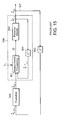
- FIG. 1 is a block diagram of a linear dynamical system, driven by white noise, whose state parameters are switched by a Markov chain model.
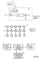
- FIG. 2 is a dependency graph illustrating a fully coupled Bayesian network representation of the SLDS of FIG. 1 .
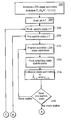
- FIG. 3 is a block diagram of an embodiment of the present invention based on approximate Viterbi inference.
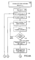
- FIGS. 4A and 4B comprise a flowchart illustrating the steps performed by the embodiment of FIG. 3 .
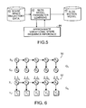
- FIG. 5 is a block diagram of an embodiment of the present invention based on approximate variational inference.
- FIG. 6 is a dependency graph illustrating the decoupling of the hidden Markov model and SLDS in the embodiment of FIG. 5 .
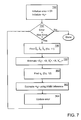
- FIG. 7 is a flowchart illustrating the steps performed by the embodiment of FIG. 5 .
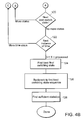
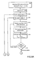
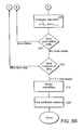
- FIGS. 8A and 8B comprise a flowchart illustrating the steps performed by a GPB2 embodiment of the present invention.
- FIG. 9 comprises two graphs which illustrate learned segmentation of a “jog” motion sequence.
- FIG. 10 is a block diagram illustrating classification of state space trajectories, as performed by the present invention.
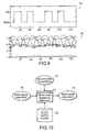
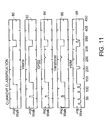
- FIG. 11 comprises several graphs which illustrate an example of segmentation.
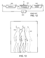
- FIG. 12 is a block diagram of a Kalman filter as employed by an embodiment of the present invention.
- FIG. 13 is a diagram illustrating the operation of the embodiment of FIG. 12 for the specific case of figure tracking.
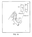
- FIG. 14 is a diagram illustrating the mapping of templates.
- FIG. 15 is a block diagram of an iterated extended Kalman filter (IEKF).
- IEEEKF extended Kalman filter
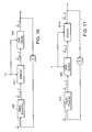
- FIG. 16 is a block diagram of an embodiment of the present invention using an IEKF in which a subset of Viterbi predictions is selected and then updated.
- FIG. 17 is a block diagram of an embodiment in which Viterbi predictions are first updated, after which a subset is selected.
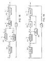
- FIG. 18 is a block diagram of an embodiment which combines SLDS prediction with sampling from a prior mixture density.
- FIG. 19 is a block diagram of an embodiment in which Viterbi estimates are combined with updated samples drawn from a prior density.
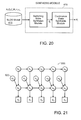
- FIG. 20 is a block diagram illustrating an embodiment of the present invention in which the framework for synthesis of state space trajectories in which an SLDS model is used as a generative model.
- FIG. 21 is a dependency graph of an SLDS model, modified according to an embodiment of the present invention, with added continuous state constraints.
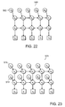
- FIG. 22 is a dependency graph of an SLDS model, modified according to an embodiment of the present invention, with added switching state constraints.
- FIG. 23 is a dependency graph of an SLDS model, modified according to an embodiment of the present invention, with both added continuous and switching state constraints.
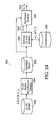
- FIG. 24 is a block diagram of the framework for a synthesis embodiment of the present invention using constraints and utilizing optimal control.
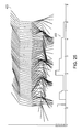
- FIG. 25 is an illustration of a stick figure motion sequence as synthesized by an embodiment of the present invention.
- FIG. 1 is a block diagram of a complex physical linear dynamic system (LDS) 10 , driven by white noise v k , also called “plant noise.”
- LDS physical linear dynamic system
- v k also called “plant noise.”
- the LDS state parameters evolve in time according to some known model, such as a Markov chain (MC) model 12 .
- MC Markov chain
- x t+1 A ( s t+1 ) x t +v t+1 ( s t+1 ),
- x t ⁇ N denotes the hidden state of the LDS 10 at time t
- v t is the state noise process
- y t ⁇ M is the observed measurement at time t
- w t is the measurement noise.
- Parameters A and C are the typical LDS parameters: the state transition matrix 14 and the observation matrix 16 , respectively. Assuming the LDS models a Gauss-Markov process, the noise processes are independently distributed Gaussian:
- the switching model 12 is assumed to be a discrete first-order Markov process. State variables of this model are written as s t . They belong to the set of S discrete symbols ⁇ e 0 , . . . , e S ⁇ 1 ⁇ , where e i is, for example, the unit vector of dimension S with a non-zero element in the i-th position.
- the switching model 12 is a first-order discrete Markov model defined with the state transition matrix ⁇ whose elements are
- switching state s t determines which of S possible models ⁇ (A 0 ,Q 0 ), . . . , (A S ⁇ 1 ,Q S ⁇ 1 ) ⁇ is used at time t.
- FIG. 2 is a dependency graph 20 equivalently illustrating a rather simple but fully coupled Bayesian network representation of the SLDS, where each s t denotes an instance of one of the discrete valued action states which switch the physical system models having continuous valued states x and producing observations y.
- s 0 ) ⁇ ⁇ t 1 T - 1 ⁇ Pr ⁇ ( x t
- x t - 1 , s t ) ⁇ ⁇ t 0 T - 1 ⁇ Pr ⁇ ( y t
- Y T , X T , and S T denote the sequences, of length T, of observation and hidden state variables, and switching variables, respectively.
- Y T ⁇ y 0 , . . . , y T ⁇ 1 ⁇ .
- the coupling between the switching states and the LDS states is full, i.e., switching states are time-dependent, LDS states are time-dependent, and switching and LDS states are intradependent.
- the goal of inference in SLDSs is to estimate the posterior probability of the hidden states of the system (s t and x t ) given some known sequence of observations Y T and the known model parameters, i.e., the likelihood of a sequence of models as well as the estimates of states. Namely, we need to find the posterior
- FIG. 3 is a block diagram of an embodiment of a dynamics learning method based on approximate Viterbi inference.
- switching dynamics of a number of SLDS motion models are learned from a corpus of state space motion examples 30 .
- Parameters 36 of each SLDS are re-estimated, at step 34 , iteratively so as to minimize the modeling cost of current state sequence estimates, obtained using the approximate Viterbi inference procedure.
- Approximate Viterbi inference is developed as an alternative to computationally expensive exact state sequence estimation.
- the task of the Viterbi approximation approach of the present invention is to find the most likely sequence of switching states s t for a given observation sequence Y T If the best sequence of switching states is denoted S* T , then the desired posterior P(X T , S T
- the switching sequence posterior at time t can be recursively computed from the same at time t ⁇ 1.
- t ⁇ 1,i,j are the likelihood associated with the transition j ⁇ i from t ⁇ 1 to t, and the probability of discrete SLDS switching from j to i.
- t,i is the “best” filtered LDS state estimate at t when the switch is in state i at time t and a sequence of t measurements, Y t , has been processed;
- t,i,j are the one-step predicted LDS state and the “best” filtered state estimates at time t, respectively, given that the switch is in state i at time t and in state j at time t ⁇ 1 and only t ⁇ 1 measurements are known.
- t,i,j ⁇ , where i and j take on all possible values, are examples of “sets of continuous state estimates.”
- t ⁇ 1,i,j ⁇ is obtained through “Viterbi prediction.” Similar definitions are easily obtained for filtered and predicted state variance estimates, ⁇ t
- transition j ⁇ i it is now easy to establish relationship between the filtered and the predicted estimates. From the theory of Kalman estimation, it follows that for transition j ⁇ i the following time updates hold:
- K i,j is the Kalman gain matrix associated with the transition j ⁇ i.
- t,i ⁇ circumflex over (x) ⁇ t
- t,i ⁇ t
- FIGS. 4A and 4B comprise a flowchart that summarizes an embodiment of the present invention employing the Viterbi inference algorithm for SLDSs, as described above.
- the steps are as follows: Initialize ⁇ ⁇ LDS ⁇ ⁇ state ⁇ ⁇ estimates ⁇ ⁇ x ⁇ 0
- FIG. 5 is a block diagram for an embodiment of the dynamics learning method based on approximate variational inference.
- reference numbers 40 - 46 correspond to reference numbers 30 - 36 of FIG. 3, the approximate Viterbi inference block 34 of FIG. 3 being replaced by the approximate variational inference block 44 .
- the switching dynamics of one or more SLDS motion models are learned from a corpus of state space motion examples 40 .
- Parameters 46 of each SLDS are re-estimated, at step 44 , iteratively so as to minimize the modeling cost of current state sequence estimates that are obtained using the approximate variational inference procedure. Approximate variational inference is developed as an alternative to computationally expensive exact state sequence estimation.
- ⁇ , Y T with an additional set of “variational parameters” h is defined such that Kullback-Leibler divergence between Q(X T , S T
- ⁇ * arg ⁇ ⁇ min ⁇ ⁇ ⁇ S t ⁇ ⁇ ⁇ X T ⁇ Q ( X T , S T
- the dependency structure of Q is chosen such that it closely resembles the dependency structure of the, original distribution P. However, unlike P, the dependency structure of Q must allow a computationally efficient inference. In our case, we define Q by decoupling the switching and LDS portions of SLDS as shown in FIG. 6 .
- FIG. 6 illustrates the factorization of the original SLDS.
- the two subgraphs of the original network are a Hidden Markov Model (HMM) Q S 50 with variational parameters ⁇ q 0 , . . . , q T ⁇ 1 ⁇ , and a time-varying LDS.
- Q X 52 with variational parameters ⁇ circumflex over (x) ⁇ 0 , ⁇ 0 , . . . , ⁇ T ⁇ 1 , ⁇ circumflex over (Q) ⁇ 0 , . . . , ⁇ circumflex over (Q) ⁇ T ⁇ 1 ⁇ .
- the two subgraphs 50 , 52 are “decoupled,” thus allowing for independent inference, Q(X T , S T
- ⁇ , Y T ) Q(X T
- ⁇ ). This is also reflected in the sufficient statistics of the posterior defined by the approximating network, e.g., (x t x′ t s t ) (x t x′ t ) (s t ).
- Equations 15 and 16 together with the inference solutions in the decoupled models form a set of fixed-point equations. Solution of this fixed-point set yields a tractable approximation to the intractable inference of the original fully coupled SLDS.
- FIG. 7 is a flowchart summarizing the variational inference algorithm for fully coupled SLDSs, corresponding to the steps below:
- Variational parameters in Equations 15 and 16 have an intuitive interpretation.
- Variational parameters of the decoupled LDS ⁇ circumflex over (Q) ⁇ t and ⁇ t in Equations 15 define a best unimodal (non-switching) representation of the corresponding switching system and are, approximately, averages of the original parameters weighted by a best estimates of the switching states P(s).
- Variational parameters of the decoupled HMM log q t (i) in Equation 16 measure the agreement of each individual LDS with the data.
- GPB2 is closely related to the Viterbi approximation described previously. It differs in that instead of picking the most likely previous switching state j at every time step t and switching state i, we collapse the M Gaussians (one for each possible value of j) into a single Gaussian.
- Regular Kalman filtering update can be used to fuse the new measurement y t and obtain S 2 new SLDS states at t for each S states at time t ⁇ 1, in a similar fashion to the Viterbi approximation embodiment discussed previously.
- GPB2 “averages” over S possible transitions from t ⁇ 1. Namely, it is easy to see that
- ⁇ circumflex over (x) ⁇ t,i,j ) ⁇ ( i, j ) Pr ( s t ⁇ 1 j
- This posterior is important because it allows one to “collapse” or “average” the S transitions into each state i into one average state, e.g. x ⁇ t
- t , i ⁇ j ⁇ x ⁇ t
- t , i , j ⁇ Pr ⁇ ( s t - 1 j
- s t i , Y t ) .
- FIGS. 8A and 8B comprise a flowchart illustrating the steps employed by a GPB2 embodiment, as summarized by the following steps:
- the inference process of the GPB2 embodiment is clearly more involved than those of the Viterbi or the variational approximation embodiments.
- GPB2 provides soft estimates of switching states at each time t.
- GPB2 is a local approximation scheme and as such does not guarantee global optimality inherent in the variational approximation.
- Xavier Boyen and Daphne Koller “Tractable inference for complex stochastic processes,” Uncertainty in Artificial Intelligence, pages 33-42, Madison, Wis., 1998, provides complex conditions for a similar type of approximation in general DBNs that lead to globally optimal solutions.
- SLDSs Learning in SLDSs can be formulated as the problem of maximum likelihood learning in general Bayesian networks.
- a generalized Expectation-Maximization (EM) algorithm can be used to find optimal values of SLDS parameters ⁇ A 0 , . . . , A s ⁇ 1 , C, Q 0 , . . . , Q s ⁇ 1 , R, ⁇ , ⁇ 0 ⁇ .
- EM Expectation-Maximization
- the EM algorithm consists of two steps, E and M, which are interleaved in an iterative fashion until convergence.
- the essential step is the expectation (E) step.
- This step is also known as the inference problem.
- the inference problem was considered in the two preferred embodiments of the method.
- the coupled E and M steps are the key components of the SLDS learning method. While the M step is the same for all preferred embodiments of the method, the E-step will vary with the approximate inference method.
- the kinematics of the figure are represented by a 2-D Scaled Prismatic Model (SPM).
- SPM Scaled Prismatic Model
- the SPM lies in the image plane, with each link having one degree of freedom (DOF) in rotation and another DOF in length.
- DOF degree of freedom
- a chain of SPM transforms can model the image displacement and foreshortening effects produced by 3-D rigid links.
- the appearance of each link in the image is described by a template of pixels which is manually initialized and deformed by the link's DOFs.
- the first task we addressed was learning an SLDS model for walking and running.
- the training set consisted of eighteen sequences of six individuals jogging and walking at a moderate pace. Each sequence was approximately fifty frames in duration.
- the training data consisted of the joint angle states of the SPM in each image frame, which were obtained manually.
- the two motion types were each modeled as multi-state SLDSs and then combined into a single complex SLDS.
- Initial state segmentation within each motion type was obtained using unsupervised clustering in a state space of some simple dynamics model, e.g., a constant velocity model. Parameters of the model (A, Q, R, x 0 , P, ⁇ 0 ) were then reestimated using the EM-learning framework with approximate Viterbi inference. This yielded refined segmentation of switching states within each of the models.
- FIG. 9 illustrates learned segmentation of a “jog” motion sequence.
- a two-state SLDS model was learned from a set of exemplary “jog” motion measurement sequences, an example of which is shown in the bottom graph.
- the top graph 62 depicts decoded switching states ((s t )) inferred from the measurement sequence y t , shown in the bottom graph 64 , using the learned “jog” SLDS model.
- the task of classification is to segment a state space trajectory into a sequence of motion regimes, according to learned models. For instance, in gesture recognition, one can automatically label portions of a long hand trajectory as some predefined, meaningful gestures.
- the SLDS framework is particularly suitable for motion trajectory classification.
- FIG. 10 illustrates the classification of state space trajectories. Learned SLDS model parameters are used in approximate Viterbi inference 74 to decode a best sequence 78 of models 76 corresponding to the state space trajectory 70 to be classified.
- the classification framework follows directly from the framework for approximate Viterbi inference in SLDSs, described previously. Namely, the approximate Viterbi inference 74 yields a sequence of switching states S T (regime indexes) 70 that best describes the observed state space trajectory 70 , assuming some current SLDS model parameters. If those model parameters are learned on a corpus of representative motion data, applying the approximate Viterbi inference on a state trajectory from the same family of motions will then result in its segmentation into the learned motion regimes.
- Additional “constraints” 72 can be imposed on classification.
- constraints 72 can model expert knowledge about the domain of trajectories which are to be classified, such as domain grammars, which may not have been present during SLDS model learning. For instance, we may know that out of N available SLDS motion models, only M ⁇ N are present in the unclassified data. We may also know that those M models can only occur in some particular, e.g., deterministically or stochastically, known order. These classification constraints can then be superimposed on the SLDS motion model parameters in the approximate Viterbi inference to force the classification to adhere to them. Hence, a number of natural language modeling techniques from human speech recognition, for example, as discussed in Jelinek, “Statistical methods for speech recognition,” MIT Press, 1998, can be mapped directly into the classification SLDS domain.
- Classification can also be performed using variational and GPB2 inference techniques. Unlike with Viterbi inference, these embodiments yield a “soft” classification, i.e., each switching state at every time instance can be active with some potentially non-zero probability.
- FIG. 11 illustrates an example of segmentation, depicting true switching state sequence (sequence of jog-walk motions) in the top graph, followed by HMM, Viterbi, GPB2, and variational state estimates using one switching state per motion type models first order SLDS model.
- FIG. 11 contains several graphs which illustrate the impact of different learned models and inference methods on classification of “jog” and “walk” motion sequences, where learned “jog” and “walk” motion models have two switching states each.
- Continuous system states of the SLDS model contain information about angle of the human figure joints.
- the top graph 80 depicts correct classification of a motion sequence containing “jog” and “walk” motions (measurement sequence is not shown).
- the remaining graphs 82 - 88 show inferred classifications using, respectively from top to bottom, SLDS model with Viterbi inference, SLDS model with GPB2 inference, SLDS model with variational inference, and HMM model.
- the SLDS learning framework can improve the tracking of target objects with complex dynamical behavior, responsive to a sequence of measurements.
- a particular embodiment of the present invention tracks the motion of the human figure, using frames from a video sequence.
- Tracking systems generally have three identifiable steps: state prediction, measurement processing and posterior update. These steps are exemplified by the well-known Kalman Filter, described in Anderson and Moore, “Optimal Filtering,” Prentice Hall, 1979.
- FIG. 12 is a standard block diagram for a Kalman Filter.
- a state prediction module 500 takes as input the state estimate from the previous time instant, ⁇ circumflex over (x) ⁇ t ⁇ 1
- the output of the prediction module 500 is the predicted state ⁇ circumflex over (x) ⁇ t
- the measurement processing module 501 takes the predicted state, generates a corresponding predicted measurement, and combines it with the actual measurement y t to form the “innovation” z t .
- states might be parameters such as angles, lengths and positions of objects or features, while the measurements might be the actual pixels.
- the predicted measurements might then be the predictions of pixel values and/or pixel locations.
- the innovation Z t measures the difference between the predicted and actual measurement data.
- the innovation z t is passed to the posterior update module 502 along with the prediction. They are fused using the Kalman gain matrix to form the posterior estimate ⁇ circumflex over (x) ⁇ t
- the delay element 503 indicates the temporal nature of the tracking process. It models the fact that the posterior estimate for the current frame becomes the input for the filter in the next frame.
- FIG. 13 illustrates the operation of the prediction module 500 for the specific case of figure tracking.
- the dashed line 510 shows the position of a skeletal representation of the human figure at time t ⁇ 1.
- the predicted position of the figure at time t is shown as a solid line 511 .
- the actual position of the figure in the video frame at time t is shown as a dotted line 512 .
- the unknown state x t represents the actual skeletal position for the sketched figure.
- a template is a region of pixels, often rectangular in shape. Tracking using template features is described in detail in James M. Rehg and Andrew P. Witkin, “Visual Tracking with Deformation Models,” Proceedings of IEEE Conference on Robotics and Automation, April 1991, Sacramento Calif., pages 844-850.
- a pixel template is associated with each part of the figure model, describing its image appearance.
- the pixel template is an example of an “image feature model” which describes the measurements provided by the image.
- two templates can be used to describe the right arm, one for the lower and one for the upper arm.
- These templates along with those for the left arm and the torso, describe the appearance of the subject's shirt.
- These templates can be initialized, for example, by capturing pixels from the first frame of the video sequence in which each part is visible.
- the use of pixel templates in figure tracking is described in detail in Daniel D. Morris and James M. Rehg, “Singularity Analysis for Articulated Object Tracking,” Proceedings of the IEEE Conference on Computer Vision and Pattern Recognition, June 1998, Santa Barbara Calif., pages 289-296.
- the innovation is the difference between the template pixel values and the pixel values in the input video frame which correspond to the predicted template position.
- the innovation function that gives the pixel difference as a function of the state vector x and pixel index k:
- Equations 18 defines a vector of pixel differences, z t , formed by subtracting pixels in the template model T from a region of pixels in the input video frame I t under the action of the figure state.
- z t a vector of pixel differences
- the contents of the template T(k) could be, for example, gray scale pixel values, color pixel values in RGB or YUV, Laplacian filtered pixels, or in general any function applied to a region of pixels.
- z(x) to denote the vector of pixel differences described by Equation (e1). Note that z t does not define an innovation process in the strict sense of the Kalman filter, since the underlying system is nonlinear and non-Gaussian.
- the deformation function pos(x,k) in Equation 17 gives the position of the kth template pixel, with respect to the input video frame, as a function of the model state x.
- t ⁇ 1 *) maps the template pixels into the current image, thereby selecting a subset of pixel measurements.
- the pos( ) function models the kinematics of the figure, which determine the relative motion of its parts.
- FIG. 14 illustrates two templates 513 and 514 which model the right arm 525 . Pixels that make up these templates 513 , 514 are ordered, with pixels T 1 through T 100 belonging to the upper arm template 513 , and pixels T 101 through T 200 belonging to the lower arm template 514 .
- the mapping pos(x,k) is also illustrated.
- the location of each template 513 , 514 under the transformation is shown as 513 A, 514 A respectively.
- the specific transformations of two representative pixel locations, T 48 and T 181 are also illustrated.
- the boundary of the figure in the image can be expressed as a collection of image contours whose shapes can be modeled for each part of the figure model. These contours can be measured in an input video frame and the innovation expressed as the distance in the image plane between the positions of predicted and measured contour locations.
- contour features for tracking is described in detail in Demetri Terzopoulos and Richard Szeliski, “Tracking with Kalman Snakes,” which appears in “Active Vision,” edited by Andrew Blake and Alan Yuille, MIT Press, 1992, pages 3-20.
- the tracking approach outlined above applies to any set of features which can be computed from a sequence of measurements.
- each frame in an image sequence generates a set of “image feature measurements,” such as pixel values, intensity gradients, or edges.
- Tracking proceeds by fitting an “image feature model,” such as a set of templates or contours, to the set of measurements in each frame.
- a primary difficulty in visual tracking is the fact that the image feature measurements are related to the figure state only in a highly nonlinear way.
- the nonlinear function I(pos(x,*)) models this effect.
- the standard approach to addressing this nonlinearity is to use the Iterated Extended Kalman Filter (IEKF), which is described in Anderson and Moore, section 8.2.
- the nonlinear measurement model in Equation 17 is linearized around the state prediction ⁇ circumflex over (x) ⁇ t
- Equation 19 The first term on the right in Equation 19, ⁇ I t (pos(x t k))′, is the image gradient ⁇ I t , evaluated at the image position of template pixel k.
- M t (x,k) is a 1 ⁇ N row vector.
- M t (x) the M ⁇ N matrix formed by stacking up these rows for each of the M pixels in the template model.
- L t is the appropriate Kalman gain matrix formed using ⁇ overscore (C) ⁇ t .
- FIG. 15 illustrates a block diagram of the IEKF.
- the measurement processing 501 and posterior update 502 blocks within the dashed box 506 are now iterated P times with the same measurement y t , for some predetermined number P, before the final output 507 is reported and a new measurement y t is introduced.
- This iteration produces a series of innovations z t n and posterior estimates ⁇ circumflex over (x) ⁇ t
- the iterations are initialized by setting ⁇ circumflex over (x) ⁇ t
- t l ⁇ circumflex over (x) ⁇ t
- t ⁇ circumflex over (x) ⁇ t
- delays 503 and 504 may be the same piece of hardware and/or software.
- the quality of the IEKF solution depends upon the quality of the state prediction.
- the linearized approximation is only valid within a small range of state values around the current operating point, which is initialized by the prediction. More generally, there are likely to be many background regions in a given video frame that are similar in appearance to the figure. For example, a template that describes the appearance of a figure wearing a dark suit might match quite well to a shadow cast against a wall in the background.
- the innovation function defined in Equation 17 can be viewed as an objective function to be minimized with respect to x. It is clear that this function will in general have many local minima. The presence of local minima poses problems for any iterative estimation technique such as IEKF.
- An accurate prediction can reduce the likelihood of becoming trapped in a local minima by bringing the starting point for the iterations closer to the correct answer.
- the SLDS framework of the present invention can describe complex dynamics as a switched sequence of linear models.
- This framework can form an accurate predictor for video tracking.
- a straightforward implementation of this approach can be extrapolated directly from the approximate Viterbi inference.
- the Viterbi approach generates a set of S 2 hypotheses, corresponding to all possible transitions i, j between linear models from time step t ⁇ 1 to t.
- Each of these hypotheses represents a prediction for the continuous state of the figure which selects a corresponding set of pixel measurements. It follows that each hypothesis has a distinct innovation equation:
- Equation 17 the only difference in comparison to Equations 18 is the use of the SLDS prediction in mapping templates into the image plane.
- This embodiment using SLDS models, is an application of the Viterbi inference algorithm described earlier to the particular measurement models used in visual tracking.
- FIG. 16 is a block diagram which illustrates this approach.
- the Viterbi prediction block 510 generates the set of S 2 predictions ⁇ circumflex over (x) ⁇ t
- a selector 511 takes these inputs and selects, for each of the S possible switching states at time t, the most likely previous state ⁇ t ⁇ 1,i , as defined in Equation 13. This step is identical to the Viterbi inference procedure described earlier, except that the likelihood of the measurement sequence is computed using image features such as templates or contours. More specifically, Equation 7 expresses the transition likelihood J t
- the measurement probability can be written
- t ⁇ 1,i,j ) P ( y t
- Equations 23 and 12 The difference between Equations 23 and 12 is the use of the linearized measurement model for template features. By changing the measurement probability appropriately, the SLDS framework above can be adopted to any tracking problem.
- the output of the selector 511 is a set of S hypotheses corresponding to the most probable state predictions given the measurement data. These are input to the IEKF update block 506 , which filters these predictions against the measurements to obtain a set of S posterior state estimates.
- This block was illustrated in FIG. 15 . This step applies the standard equations for the IEKF to features such as templates or contours, as described in Equations 17 through 21.
- the posterior estimates can be decoded and smoothed analogously to the case of Viterbi inference.
- the selector 511 In computing the measurement probabilities, the selector 511 must make S 2 comparisons between all of the model pixels and the input image. Depending upon the size of the target and the image, this may represent a large computation. This computation can be reduced by considering only the Markov process probabilities and not the measurement probabilities in computing the best S switching hypotheses. In this case, the best hypotheses are given by
- i* t arg min j ⁇ log ⁇ ( i, j )+ J t ⁇ 1,j ⁇ (Eq. 24)
- FIG. 17 illustrates a second tracking embodiment, in which the order of the IEKF update module 506 and selector 511 A is reversed.
- the set of S 2 predictions are passed directly to the IEKF update module 506 .
- the output of the update module 506 is a set of S 2 filtered estimates ⁇ circumflex over (x) ⁇ t
- the selector 511 A chooses the most likely transition j ⁇ i for each switching state based on the filtered estimates. This is analogous to the Viterbi inference case, which was described in the embodiment of FIG. 16 above.
- the key step is to compute the switching costs J t,i defined in Equations 5 and 6. The difference in this case comes from the fact that the probability of the measurement is computed using the filtered posterior estimate rather than the prediction. This probability is given by:
- t,i,j ) P ( y t
- the state j* is the “optimal posterior switching state,” and its value depends upon the posterior estimate for the continuous state at time t.
- the set of S 2 predictions used in the embodiments of FIGS. 16 and 17 can be viewed as specifying a set of starting points for local optimization of an objective function defined by ⁇ z t (x) ⁇ 2 .
- the behavior of the IEKF module 506 approaches steepest-descent gradient search because the dynamic model no longer influences the posterior estimate.
- a wide range of sampling procedures is available for generating additional starting points for search.
- a state prediction must be specified and a particular dynamic model selected. The easiest way to do this is to assume that new starting points are going to be obtained by sampling from the mixture density defined by the set of S 2 predictions.
- the first term in the summed product is a Gaussian prior density from the Viterbi inference step.
- the second term is its likelihood, a scalar probability which we denote ⁇ i,j .
- Rewriting in the form of a mixture of S 2 Gaussian kernels, i.e., the predictions, yields: P ⁇ ( x t ⁇ Y t - 1 ) ⁇ ⁇ i , j ⁇ ⁇ i , j ⁇ K i , j ⁇ ( x t ) ⁇ i , j ⁇ ⁇ i , j ⁇ N ⁇ [ x i ; x ⁇ t ⁇ t - 1 , i , j , ⁇ t ⁇ t - 1 , i , j ] ( Eq . ⁇ 26 )
- Equation 27 All of the terms in the numerator of Equation 27 are directly available from the Viterbi inference method.
- Equations 26 and 28 define a “Viterbi mixture density” from which additional starting points for search can be drawn.
- the steps for drawing R additional points are as follows:
- the rth sample is associated with a specific prediction (i r , j r ), making it easy to apply the IEKF.
- Equation 29 defines a modification of the IEKF update block to handle arbitrary starting points in computing the posterior update.
- MHT multiple hypothesis tracking
- FIG. 18 is a block diagram of a tracking embodiment which combines SLDS prediction with sampling from the prior mixture density to perform tracking.
- the output of the Viterbi predictor 510 follows two paths. The top path is similar to the embodiment of FIG. 16 .
- the predictions are processed by a selector 515 and then input to an IEKF update block 506 .
- This set is unioned with the SLDS predictions from the selector 515 and input to the IEKF block 506 .
- the output of the IEKF block 506 is a joint set of filtered estimates, corresponding to the SLDS predictions, which we now write as ⁇ overscore (x) ⁇ t
- This combined output forms the input to a final selector 519 which selects one filtered estimate for each of the switching states to make up the final output set.
- This selection process is identical to the ones described earlier with respect to FIG. 17, except that there now can be more than one possible estimate for a given state transition (i,j), corresponding to different starting points for search.
- FIG. 19 illustrates yet another tracking embodiment.
- the output of Viterbi prediction which comprises “Viterbi estimates,” is input directly to an IEKF update block 506 while the output of the sample generator 517 goes to an MHT block 520 , which implements the method of Cham and Rehg referred to above.
- these two sets of filtered estimates are passed to a final selector 522 .
- This final selector 522 chooses S of the posterior estimates, one for each possible switching state, as the final output.
- this selector uses the posterior switching costs defined in Equation 25B.
- GPB2 Generalized Psuedo Bayesian approximation
- SLDS was introduced as a “generative” model; trajectories in the state space can be easily generated by simulating an SLDS. Nevertheless, SLDSs are still more commonly employed as a classifier or a filter/predictor than as a generative model. We now formulate a framework for using SLDSs as synthesizers and interpolators.
- FIG. 20 illustrates a framework for synthesis of state space trajectories in which the SLDS is used as a generative model within a synthesis module 410 .
- a switching state sequence s t is first synthesized in the switching state synthesis module 412 by sampling from a Markoy chain with state transition probability matrix ⁇ and initial state distribution ⁇ 0 .
- the continuous state sequence x t is then synthesized in the continuous state synthesis module 413 by sampling from a LDS with parameters A(s t ), Q(s t ), C, R, x 0 (s 0 ), and Q 0 (s 0 ).
- the above procedure will produce a random sequence of samples from the SLDS model. If an average noiseless state trajectory is desired, the synthesis can be run with LDS noise parameters (Q(s t ), R, Q 0 (s 0 )) set to zero and switching states whose duration is equal to average state durations, as determined by the switching state transition matrix ⁇ . For example, this would result in sequences of prototypical walk or jog motions, whereas the random sampling would exhibit deviations from such prototypes. Intermediate levels of randomness can be achieved by scaling the SLDS model noise parameters with factors between 0 and 1.
- the model parameters can also be modified to meet new constraints that were, for instance, not present in the data used to learn the SLDS.
- initial state mean x 0 , variance Q 0 and switching state distribution ⁇ can be changed so as to force the SLDS to start in some arbitrary state x a of regime i a , e.g., to start simulation in a “walking” regime i a with figure posture x a .
- a framework of optimal control can be used to formalize synthesis under constraints.
- Optimal control of linear dynamic systems is described, for example, in B. Anderson and J. Moore, “Optimal Control: Linear Quadratic Methods,” Prentice Hall, Englewood Cliffs, N.J., 1990.
- the optimal control framework provides a way to design an optimal input or control u t to the LDS, such that the LDS state x t gets as close as possible to a desired state x t d .
- the desired states can also be viewed as constraint points.
- Equation 1 can be modified as
- FIG. 21 is a dependency graph of the modified SLDS 550 with added controls u t 552 .
- a goal is to find u t that makes x t as close as possible to a given x t d .
- W t (x) and W t (u) are weight matrices.
- x t d might correspond to a desired figure posture at key frame t
- W t (x) might designate the key frame, i.e., W t (x) is large for the key frame, and small otherwise.
- constraints that can be cast in this framework are the inequality or bounding constraints on the state x t or control u t (e.g., x t >x min , u t ⁇ u max ). Such constraints could prevent, for example, the limbs of a simulated human figure from assuming physically unrealistic postures, or the control u t from becoming unrealistically large.
- the solution for the best control u t can be derived using the framework of linear quadratic regulators (LQR) for time-varying LDS.
- LQR linear quadratic regulators
- the SLDS 560 can be modified to include inputs 562 , i.e., controls, to the switching state.
- the modified SLDS 560 is then described by the following equation:
- Pr ( s t+1 i
- ⁇ (a) (i,j,k) defines a conditioned switching state transition matrix which depends on the control a t 562 .
- constraints imposed on the switching states can be satisfied.
- constraints can be formulated similarly to constraints for the continuous control input of FIG. 21, e.g., switching state constraints, switching input constraints and minimum-time constraints.
- a switching state constraint can guarantee that a figure is in the walking motion regime from time t s to t e .
- To find an optimal control â t that satisfies those constraints one would have to use a modified value function that includes the cost of the switching state control.
- a framework for the switching state optimal control could be derived from the theory of reinforcement learning and Markov decision processes. See, for example, Sutton, R. S. and Barto, A. G., “Reinforcement Learning: An Introduction,” Cambridge, Mass., MIT Press, 1998.
- c t (s t ,s t ⁇ 1 ,a t ) represents a cost for making the transition from switching state s t ⁇ 1 to s t , for a given control a t
- ⁇ is a discount or “forgetting” factor.
- the cost function c t is designed to emphasize, with a low c t , those states that agree with imposed constraints, and to penalize, with a high c t , those states that violate the imposed constraints.
- the SLDS system 750 can be modified to include both types of controls, continuous 572 and switching 574 , as indicated by the following equation.
- x t+1 A ( s t+1 ) x t +u t+1 +v ( s t+1 )
- the mixed control (u t , a t ) can lead to both a desired switching state, e.g., motion regime, and a desired continuous state, e.g., figure posture.
- a constraint can be specified that requires the human figure to be in the walking regime i d with some specific posture x d at time t.
- additional constraints such as input bounding and minimum time can also be specified for the mixed state control.
- a value function can be used that includes the costs of the switching and the continuous state controls, e.g., V (x) +V (s) .
- the modified generative SLDS model can be used to produce a synthetic trajectory.
- FIG. 24 illustrates the framework 580 , for synthesis under constraints, which utilizes optimal control.
- the SLDS model 582 is modified by a SLDS model modification module 584 to include the control terms or inputs.
- an optimal control module 586 finds the optimal controls 587 which satisfy constraints 588 .
- a synthesis model 590 generates synthesized trajectories 592 from the modified SLDS 585 and the optimal controls 587 .
- the spacetime approach can be extended to include the direct use of motion capture data. This is described in Michael Gleicher, “Retargetting Motion to New Characters,” Proceedings of SIGGRAPH 98, in Computer Graphics Proceedings, Annual Conference series, 1998, pages 33-42.
- a single sequence of human motion data is modified to achieve a specific animation objective by filtering it with a biomechanical model of human motion and adjusting the model parameters.
- a motion sequence of a person walking can be adapted to a figure model whose proportions are different from that of the subject.
- Motions can also be modified to satisfy various equality or inequality constraints.
- our framework employs a set of LDS models to describe feature data, resulting in models with much more expressive power.
- the prior art does not describe any mechanism for imposing constraints on the samples from the models. This may make it difficult to use this approach in achieving specific animation objectives.
- the learned walk/jog SLDS was used to generate a “synthetic walk” based on initial conditions learned by the SLDS model.
- FIG. 25 illustrates a stick FIG. 220 motion sequence of the noise driven model.
- the stick figure exhibits more or less “natural”-looking walk. Departure from the realistic walk becomes more evident as the simulation time progresses. This behavior is not unexpected as the SLDS in fact learns locally consistent motion patterns.
- FIG. 25 illustrates a synthesized walk motion over 50 frames using SLDS as a generative model. The states of the synthesized motion are shown on the graph 222 .
- Our invention makes possible a number of core tasks related to the analysis and synthesis of the human figure motion:
- Interfaces based on vision sensing could benefit from improved tracking and better classification performance due to the SLDS approach.
- Motion capture in unstructured environments can be enabled through better tracking techniques. In addition to the capture of live motion without the use of special clothing, it is also possible to capture motion from archival sources such as old movies.
- Motion synthesis The generation of human motion for computer graphics animation can be enabled through the use of a learned, generative stochastic model. By learning models from sample motions, it is possible to capture the natural dynamics implicit in real human motion without a laborious manual modeling process. Because the resulting models are stochastic, sampling from the models produces motion with a pleasing degree of randomness.
- Video editing Tracking algorithms based on powerful dynamic models can simplify the task of segmenting video sequences.
- Video compression/decompression The ability to interpolate a video sequence based on a sparse set of samples could provide a new approach to coding and decoding video sequences containing human or other motion. In practice, human motion is common in video sequences. By transmitting key frames detected using SLSD classification at a low sampling rate and interpolating, using SLDS interpolation, the missing frames from the transmitted model parameters, a substantial savings in bit-rate may be achievable.
- a computer usable medium can include a readable memory device, such as a hard drive device, a CD-ROM, a DVD-ROM, or a computer diskette, having computer readable program code segments stored thereon.
- the computer readable medium can also include a communications or transmission medium, such as a bus or a communications link, either optical, wired, or wireless, having program code segments carried thereon as digital or analog data signals.
Abstract
Description


Claims (1)
Priority Applications (2)
| Application Number | Priority Date | Filing Date | Title |
|---|---|---|---|
| US09/654,022 US6683968B1 (en) | 1999-09-16 | 2000-09-01 | Method for visual tracking using switching linear dynamic system models |
| US10/662,067 US6999601B2 (en) | 1999-09-16 | 2003-09-12 | Method for visual tracking using switching linear dynamic systems models |
Applications Claiming Priority (2)
| Application Number | Priority Date | Filing Date | Title |
|---|---|---|---|
| US15438499P | 1999-09-16 | 1999-09-16 | |
| US09/654,022 US6683968B1 (en) | 1999-09-16 | 2000-09-01 | Method for visual tracking using switching linear dynamic system models |
Related Child Applications (1)
| Application Number | Title | Priority Date | Filing Date |
|---|---|---|---|
| US10/662,067 Continuation US6999601B2 (en) | 1999-09-16 | 2003-09-12 | Method for visual tracking using switching linear dynamic systems models |
Publications (1)
| Publication Number | Publication Date |
|---|---|
| US6683968B1 true US6683968B1 (en) | 2004-01-27 |
Family
ID=30117767
Family Applications (2)
| Application Number | Title | Priority Date | Filing Date |
|---|---|---|---|
| US09/654,022 Expired - Fee Related US6683968B1 (en) | 1999-09-16 | 2000-09-01 | Method for visual tracking using switching linear dynamic system models |
| US10/662,067 Expired - Lifetime US6999601B2 (en) | 1999-09-16 | 2003-09-12 | Method for visual tracking using switching linear dynamic systems models |
Family Applications After (1)
| Application Number | Title | Priority Date | Filing Date |
|---|---|---|---|
| US10/662,067 Expired - Lifetime US6999601B2 (en) | 1999-09-16 | 2003-09-12 | Method for visual tracking using switching linear dynamic systems models |
Country Status (1)
| Country | Link |
|---|---|
| US (2) | US6683968B1 (en) |
Cited By (33)
| Publication number | Priority date | Publication date | Assignee | Title |
|---|---|---|---|---|
| US20030093245A1 (en) * | 2001-11-13 | 2003-05-15 | National Instruments Corporation | Measurement system which uses a state model |
| US20030103565A1 (en) * | 2001-12-05 | 2003-06-05 | Lexing Xie | Structural analysis of videos with hidden markov models and dynamic programming |
| US20040186718A1 (en) * | 2003-03-19 | 2004-09-23 | Nefian Ara Victor | Coupled hidden markov model (CHMM) for continuous audiovisual speech recognition |
| US20050111753A1 (en) * | 2003-11-20 | 2005-05-26 | Yissum Research Development Company Of The Hebrew University Of Jerusalem | Image mosaicing responsive to camera ego motion |
| US20050175219A1 (en) * | 2003-11-13 | 2005-08-11 | Ming-Hsuan Yang | Adaptive probabilistic visual tracking with incremental subspace update |
| US20050195102A1 (en) * | 2004-03-05 | 2005-09-08 | Vaman Dhadesugoor R. | Real time predictive trajectory pairing (RTPTP) algorithm for highly accurate tracking of ground or air moving objects |
| US20050277466A1 (en) * | 2004-05-26 | 2005-12-15 | Playdata Systems, Inc. | Method and system for creating event data and making same available to be served |
| WO2006010129A2 (en) * | 2004-07-09 | 2006-01-26 | Honda Motor Co., Ltd. | Adaptive discriminative generative model and incremental fisher discriminant analysis and application to visual tracking |
| US7092924B1 (en) * | 2002-02-28 | 2006-08-15 | Raytheon Company | Method and system for assigning observations |
| US20060285770A1 (en) * | 2005-06-20 | 2006-12-21 | Jongwoo Lim | Direct method for modeling non-rigid motion with thin plate spline transformation |
| US7187320B1 (en) * | 2004-08-27 | 2007-03-06 | Lockheed Martin Corporation | Matched maneuver detector |
| US20070255454A1 (en) * | 2006-04-27 | 2007-11-01 | Honda Motor Co., Ltd. | Control Of Robots From Human Motion Descriptors |
| US20080007446A1 (en) * | 2006-07-04 | 2008-01-10 | Denso Corporation | Radar device |
| US20100030539A1 (en) * | 2008-08-01 | 2010-02-04 | Sundeep Chandhoke | Simulation of a Motion System Including a Mechanical Modeler with Interpolation |
| US20100208941A1 (en) * | 2009-02-13 | 2010-08-19 | Broaddus Christopher P | Active coordinated tracking for multi-camera systems |
| US20100299145A1 (en) * | 2009-05-22 | 2010-11-25 | Honda Motor Co., Ltd. | Acoustic data processor and acoustic data processing method |
| US20100295783A1 (en) * | 2009-05-21 | 2010-11-25 | Edge3 Technologies Llc | Gesture recognition systems and related methods |
| US20120219184A1 (en) * | 2009-08-06 | 2012-08-30 | Kabushiki Kaisha Toshiba | Monitoring of video images |
| US20130013112A1 (en) * | 2010-02-25 | 2013-01-10 | Honda Motor Co., Ltd. | Constrained Resolved Acceleration Control |
| US8396252B2 (en) | 2010-05-20 | 2013-03-12 | Edge 3 Technologies | Systems and related methods for three dimensional gesture recognition in vehicles |
| US8467599B2 (en) | 2010-09-02 | 2013-06-18 | Edge 3 Technologies, Inc. | Method and apparatus for confusion learning |
| US8582866B2 (en) | 2011-02-10 | 2013-11-12 | Edge 3 Technologies, Inc. | Method and apparatus for disparity computation in stereo images |
| US8655093B2 (en) | 2010-09-02 | 2014-02-18 | Edge 3 Technologies, Inc. | Method and apparatus for performing segmentation of an image |
| US8666144B2 (en) | 2010-09-02 | 2014-03-04 | Edge 3 Technologies, Inc. | Method and apparatus for determining disparity of texture |
| US8705877B1 (en) | 2011-11-11 | 2014-04-22 | Edge 3 Technologies, Inc. | Method and apparatus for fast computational stereo |
| US8970589B2 (en) | 2011-02-10 | 2015-03-03 | Edge 3 Technologies, Inc. | Near-touch interaction with a stereo camera grid structured tessellations |
| US9152880B1 (en) * | 2014-05-30 | 2015-10-06 | The United States Of America As Represented By The Secretarty Of The Army | Method for modeling human visual discrimination task performance of dynamic scenes |
| US20160161606A1 (en) * | 2014-12-08 | 2016-06-09 | Northrop Grumman Systems Corporation | Variational track management |
| US9519049B1 (en) * | 2014-09-30 | 2016-12-13 | Raytheon Company | Processing unknown radar emitters |
| US20180114094A1 (en) * | 2016-10-26 | 2018-04-26 | Freescale Semiconductor, Inc. | Method and apparatus for data set classification based on generator features |
| US20180181543A1 (en) * | 2016-12-27 | 2018-06-28 | David Levin | Method and apparatus for the sensor-independent representation of time-dependent processes |
| US10242447B2 (en) | 2016-09-08 | 2019-03-26 | Sony Corporation | Video processing system and method for deformation and occlusion resistant object tracking in video content |
| US10721448B2 (en) | 2013-03-15 | 2020-07-21 | Edge 3 Technologies, Inc. | Method and apparatus for adaptive exposure bracketing, segmentation and scene organization |
Families Citing this family (20)
| Publication number | Priority date | Publication date | Assignee | Title |
|---|---|---|---|---|
| US6822653B2 (en) * | 2002-06-28 | 2004-11-23 | Microsoft Corporation | Methods and system for general skinning via hardware accelerators |
| EP1569570B1 (en) * | 2002-11-27 | 2006-11-15 | Medical Device Innovations Limited | Tissue ablation apparatus |
| US20050228673A1 (en) * | 2004-03-30 | 2005-10-13 | Nefian Ara V | Techniques for separating and evaluating audio and video source data |
| US7720257B2 (en) * | 2005-06-16 | 2010-05-18 | Honeywell International Inc. | Object tracking system |
| EP1916538A3 (en) * | 2006-10-27 | 2011-02-16 | Panasonic Electric Works Co., Ltd. | Target moving object tracking device |
| TWI328201B (en) * | 2006-10-30 | 2010-08-01 | Ind Tech Res Inst | Method and system for object detection in an image plane |
| US8154600B2 (en) * | 2007-04-20 | 2012-04-10 | Utc Fire & Security Americas Corporation, Inc. | Method and system for distributed multiple target tracking |
| EP2153370B1 (en) * | 2007-05-03 | 2017-02-15 | Motek B.V. | Method and system for real time interactive dynamic alignment of prosthetics |
| US8432449B2 (en) * | 2007-08-13 | 2013-04-30 | Fuji Xerox Co., Ltd. | Hidden markov model for camera handoff |
| EP2209018A1 (en) * | 2009-01-15 | 2010-07-21 | Nederlandse Organisatie voor toegepast-natuurwetenschappelijk Onderzoek TNO | A method for estimating an object motion characteristic from a radar signal, a computer system and a computer program product |
| US8213680B2 (en) * | 2010-03-19 | 2012-07-03 | Microsoft Corporation | Proxy training data for human body tracking |
| EP2474950B1 (en) * | 2011-01-05 | 2013-08-21 | Softkinetic Software | Natural gesture based user interface methods and systems |
| US8478711B2 (en) | 2011-02-18 | 2013-07-02 | Larus Technologies Corporation | System and method for data fusion with adaptive learning |
| US8774499B2 (en) | 2011-02-28 | 2014-07-08 | Seiko Epson Corporation | Embedded optical flow features |
| US9665767B2 (en) * | 2011-02-28 | 2017-05-30 | Aic Innovations Group, Inc. | Method and apparatus for pattern tracking |
| US8892491B2 (en) | 2011-11-21 | 2014-11-18 | Seiko Epson Corporation | Substructure and boundary modeling for continuous action recognition |
| CN104516905B (en) * | 2013-09-29 | 2020-11-06 | 日电(中国)有限公司 | Method and device for mining rare balanced trajectory data |
| JP6402611B2 (en) * | 2014-12-04 | 2018-10-10 | 富士通株式会社 | Input control method, input control program, and information processing apparatus |
| CN109344755B (en) * | 2018-09-21 | 2024-02-13 | 广州市百果园信息技术有限公司 | Video action recognition method, device, equipment and storage medium |
| CN111938655B (en) * | 2020-07-09 | 2021-09-03 | 上海交通大学 | Orbit soft tissue form evaluation method, system and equipment based on key point information |
Citations (10)
| Publication number | Priority date | Publication date | Assignee | Title |
|---|---|---|---|---|
| US5325098A (en) * | 1993-06-01 | 1994-06-28 | The United States Of America As Represented By The Secretary Of The Navy | Interacting multiple bias model filter system for tracking maneuvering targets |
| US5923712A (en) * | 1997-05-05 | 1999-07-13 | Glenayre Electronics, Inc. | Method and apparatus for linear transmission by direct inverse modeling |
| US6064703A (en) | 1996-07-29 | 2000-05-16 | Telital S.P.A. | MAP receiver for high-speed numerical transmissions through rayleigh channels noisy and dispersive in time and frequency |
| US6226409B1 (en) * | 1998-11-03 | 2001-05-01 | Compaq Computer Corporation | Multiple mode probability density estimation with application to sequential markovian decision processes |
| US6243037B1 (en) * | 1995-12-19 | 2001-06-05 | The Commonwealth Of Australia | Tracking method for a radar system |
| US6256418B1 (en) * | 1998-04-13 | 2001-07-03 | Compaq Computer Corporation | Method and system for compressing a sequence of images including a moving figure |
| US6314204B1 (en) | 1998-11-03 | 2001-11-06 | Compaq Computer Corporation | Multiple mode probability density estimation with application to multiple hypothesis tracking |
| US6393046B1 (en) * | 1996-04-25 | 2002-05-21 | Sirf Technology, Inc. | Spread spectrum receiver with multi-bit correlator |
| US6396878B1 (en) * | 1997-02-28 | 2002-05-28 | Nokia Telecommunications Oy | Reception method and a receiver |
| US6480876B2 (en) * | 1998-05-28 | 2002-11-12 | Compaq Information Technologies Group, L.P. | System for integrating task and data parallelism in dynamic applications |
Family Cites Families (3)
| Publication number | Priority date | Publication date | Assignee | Title |
|---|---|---|---|---|
| US5243037A (en) * | 1990-09-21 | 1993-09-07 | E. I. Du Pont De Nemours And Company | Poly(fluoroalkyl) sugar reagents for surface modification of supports |
| TW413795B (en) | 1999-02-26 | 2000-12-01 | Cyberlink Corp | An image processing method of 3-D head motion with three face feature points |
| US6591146B1 (en) | 1999-09-16 | 2003-07-08 | Hewlett-Packard Development Company L.C. | Method for learning switching linear dynamic system models from data |
-
2000
- 2000-09-01 US US09/654,022 patent/US6683968B1/en not_active Expired - Fee Related
-
2003
- 2003-09-12 US US10/662,067 patent/US6999601B2/en not_active Expired - Lifetime
Patent Citations (10)
| Publication number | Priority date | Publication date | Assignee | Title |
|---|---|---|---|---|
| US5325098A (en) * | 1993-06-01 | 1994-06-28 | The United States Of America As Represented By The Secretary Of The Navy | Interacting multiple bias model filter system for tracking maneuvering targets |
| US6243037B1 (en) * | 1995-12-19 | 2001-06-05 | The Commonwealth Of Australia | Tracking method for a radar system |
| US6393046B1 (en) * | 1996-04-25 | 2002-05-21 | Sirf Technology, Inc. | Spread spectrum receiver with multi-bit correlator |
| US6064703A (en) | 1996-07-29 | 2000-05-16 | Telital S.P.A. | MAP receiver for high-speed numerical transmissions through rayleigh channels noisy and dispersive in time and frequency |
| US6396878B1 (en) * | 1997-02-28 | 2002-05-28 | Nokia Telecommunications Oy | Reception method and a receiver |
| US5923712A (en) * | 1997-05-05 | 1999-07-13 | Glenayre Electronics, Inc. | Method and apparatus for linear transmission by direct inverse modeling |
| US6256418B1 (en) * | 1998-04-13 | 2001-07-03 | Compaq Computer Corporation | Method and system for compressing a sequence of images including a moving figure |
| US6480876B2 (en) * | 1998-05-28 | 2002-11-12 | Compaq Information Technologies Group, L.P. | System for integrating task and data parallelism in dynamic applications |
| US6226409B1 (en) * | 1998-11-03 | 2001-05-01 | Compaq Computer Corporation | Multiple mode probability density estimation with application to sequential markovian decision processes |
| US6314204B1 (en) | 1998-11-03 | 2001-11-06 | Compaq Computer Corporation | Multiple mode probability density estimation with application to multiple hypothesis tracking |
Non-Patent Citations (21)
| Title |
|---|
| A Brief Introduction to Graphical Models and Bayesian Networks, http://www.cs.berkeley.edu/˜murphyk/Bayes/bayes.html, pp. 1-19. |
| A Brief Introduction to Graphical Models and Bayesian Networks, http://www.cs.berkeley.edu/<~>murphyk/Bayes/bayes.html, pp. 1-19. |
| Bar-Shalom Y. Li, X-R, Estimation & Tracking: principles, techniques, and software. YBS, Storrs, CT, 1998, pp. 446-484. |
| Ghahramani, Z. and Hinton G.E., Parameter Estimation for Linear Dynamical Systems, pp. 1-6, Technical Report CRG-TR-96-2, Dept. of Computer Science, University of Toronto. |
| Ghahramani, Z., et al., Switching State-Space Models, pp. 1-23. Technical Report CRG-TR-96-3, Dept. of Computer Science, University of Toronto. |
| Ghahramani, Zoubin and Hinton, G.E., Variational Learning for Switching State-Space Models, Gatsby Computational Neuroscience Unit,, pp. 1-26. |
| http://www.scs.leeds.ac.uk/scs-only/teaching-materials/HiddenMarkovModels/html_dev/main.html. |
| Jordan, M.I., et al., An Introduction to Variational Methods for Graphical Models, Oct. 11, 1999, http://www.stat.berkeley.edu/tech-reports/index.html, Report#508. |
| Kim, Chang-Jin, Dynamic Linear Models with Markov-Switching, Journal of Econometrics 60, (1994) pp. 1-22. |
| Krishnamurthy, V. and Evans, J., Finite-Dimensional Filters for Passive Tracking of Markov Jump Linear Systems, Automatica, vol. 34, No. 6, pp. 765-770, 1998. |
| Maybeck, P.S., Stochastic Models, Estimation, and Control, vol. I Academic Press, 1979. |
| Minka, Thomas P., From Hidden Markov Models to Linear Dynamical Systems, pp. 1-10. ftp://vismod.www.media.mit.edu/pub/tpminka/papers/minka-lds-tut.ps.gz. |
| Murphy, Kevin P., Inference and Learning in Hybrid Bayesian Networks, Report No. UCB/CSD-98-990, Jan. 1998, pp. 1-18. |
| Murphy, Kevin P., Switching Kalman Filters, Aug. 21, 1998, pp. 1-16. |
| Pavlovic, Vladimir, et al., A Dynamic Bayesian Network Approach to Figure Tracking Using Learned Dynamic Models. |
| Pavlović, Vladimir, et al., A Dynamic Bayesian Network Approach to Figure Tracking Using Learned Dynamic Models. |
| Pavlovic, Vladimir, et al., Time-Series Classification Using Mixed State Dynamic Bayesian Networks, In Computer Vision and Pattern Recognition, pp. 609-615, Jun. 1999. |
| Pavlović, Vladimir, et al., Time-Series Classification Using Mixed State Dynamic Bayesian Networks, In Computer Vision and Pattern Recognition, pp. 609-615, Jun. 1999. |
| Rabiner, L.R. and Juang, B.H., An Introduction to Hidden Markov Models, IEEE ASSP Magazine, Jan. 1986, pp. 4-16. |
| Shumway, R.H. and Stoffer, D.S., Dynamic Linear Models with Switching, Journal of the American Statistical Association, Sep. 1991, vol. 86, No. 415. |
| Welch, Greg and Bishop, Gary, An Introduction to the Kalman Filter, Department of Computer Science, Univ. of North Carolina at Chapel Hill, Chapel Hill, NC 27599-3175, Sep. 17, 1997, pp. 1-16. |
Cited By (81)
| Publication number | Priority date | Publication date | Assignee | Title |
|---|---|---|---|---|
| US20030093245A1 (en) * | 2001-11-13 | 2003-05-15 | National Instruments Corporation | Measurement system which uses a state model |
| US7089141B2 (en) * | 2001-11-13 | 2006-08-08 | National Instruments Corporation | Measurement system which uses a state model |
| US6865226B2 (en) * | 2001-12-05 | 2005-03-08 | Mitsubishi Electric Research Laboratories, Inc. | Structural analysis of videos with hidden markov models and dynamic programming |
| US20030103565A1 (en) * | 2001-12-05 | 2003-06-05 | Lexing Xie | Structural analysis of videos with hidden markov models and dynamic programming |
| US7092924B1 (en) * | 2002-02-28 | 2006-08-15 | Raytheon Company | Method and system for assigning observations |
| US20040186718A1 (en) * | 2003-03-19 | 2004-09-23 | Nefian Ara Victor | Coupled hidden markov model (CHMM) for continuous audiovisual speech recognition |
| US7454342B2 (en) * | 2003-03-19 | 2008-11-18 | Intel Corporation | Coupled hidden Markov model (CHMM) for continuous audiovisual speech recognition |
| US20050175219A1 (en) * | 2003-11-13 | 2005-08-11 | Ming-Hsuan Yang | Adaptive probabilistic visual tracking with incremental subspace update |
| US7463754B2 (en) | 2003-11-13 | 2008-12-09 | Honda Motor Co. | Adaptive probabilistic visual tracking with incremental subspace update |
| US20050111753A1 (en) * | 2003-11-20 | 2005-05-26 | Yissum Research Development Company Of The Hebrew University Of Jerusalem | Image mosaicing responsive to camera ego motion |
| US20050195102A1 (en) * | 2004-03-05 | 2005-09-08 | Vaman Dhadesugoor R. | Real time predictive trajectory pairing (RTPTP) algorithm for highly accurate tracking of ground or air moving objects |
| US20050277466A1 (en) * | 2004-05-26 | 2005-12-15 | Playdata Systems, Inc. | Method and system for creating event data and making same available to be served |
| US9087380B2 (en) * | 2004-05-26 | 2015-07-21 | Timothy J. Lock | Method and system for creating event data and making same available to be served |
| US20060036399A1 (en) * | 2004-07-09 | 2006-02-16 | Ming-Hsuan Yang | Adaptive discriminative generative model and application to visual tracking |
| US20060023916A1 (en) * | 2004-07-09 | 2006-02-02 | Ming-Hsuan Yang | Visual tracking using incremental fisher discriminant analysis |
| US7369682B2 (en) | 2004-07-09 | 2008-05-06 | Honda Motor Co., Ltd. | Adaptive discriminative generative model and application to visual tracking |
| WO2006010129A3 (en) * | 2004-07-09 | 2006-03-23 | Honda Motor Co Ltd | Adaptive discriminative generative model and incremental fisher discriminant analysis and application to visual tracking |
| US7650011B2 (en) * | 2004-07-09 | 2010-01-19 | Honda Motor Co., Inc. | Visual tracking using incremental fisher discriminant analysis |
| JP2011003207A (en) * | 2004-07-09 | 2011-01-06 | Honda Motor Co Ltd | Adaptive discriminative generative model and incremental fisher discriminant analysis and application to visual tracking |
| WO2006010129A2 (en) * | 2004-07-09 | 2006-01-26 | Honda Motor Co., Ltd. | Adaptive discriminative generative model and incremental fisher discriminant analysis and application to visual tracking |
| US7187320B1 (en) * | 2004-08-27 | 2007-03-06 | Lockheed Martin Corporation | Matched maneuver detector |
| US20060285770A1 (en) * | 2005-06-20 | 2006-12-21 | Jongwoo Lim | Direct method for modeling non-rigid motion with thin plate spline transformation |
| US7623731B2 (en) | 2005-06-20 | 2009-11-24 | Honda Motor Co., Ltd. | Direct method for modeling non-rigid motion with thin plate spline transformation |
| US20070255454A1 (en) * | 2006-04-27 | 2007-11-01 | Honda Motor Co., Ltd. | Control Of Robots From Human Motion Descriptors |
| US8924021B2 (en) | 2006-04-27 | 2014-12-30 | Honda Motor Co., Ltd. | Control of robots from human motion descriptors |
| US20080007446A1 (en) * | 2006-07-04 | 2008-01-10 | Denso Corporation | Radar device |
| US8239177B2 (en) * | 2008-08-01 | 2012-08-07 | National Instruments Corporation | Simulation of a motion system including a mechanical modeler with interpolation |
| US20100030539A1 (en) * | 2008-08-01 | 2010-02-04 | Sundeep Chandhoke | Simulation of a Motion System Including a Mechanical Modeler with Interpolation |
| US8180107B2 (en) * | 2009-02-13 | 2012-05-15 | Sri International | Active coordinated tracking for multi-camera systems |
| US20100208941A1 (en) * | 2009-02-13 | 2010-08-19 | Broaddus Christopher P | Active coordinated tracking for multi-camera systems |
| US20100295783A1 (en) * | 2009-05-21 | 2010-11-25 | Edge3 Technologies Llc | Gesture recognition systems and related methods |
| US11703951B1 (en) | 2009-05-21 | 2023-07-18 | Edge 3 Technologies | Gesture recognition systems |
| US9417700B2 (en) | 2009-05-21 | 2016-08-16 | Edge3 Technologies | Gesture recognition systems and related methods |
| US8548802B2 (en) * | 2009-05-22 | 2013-10-01 | Honda Motor Co., Ltd. | Acoustic data processor and acoustic data processing method for reduction of noise based on motion status |
| US20100299145A1 (en) * | 2009-05-22 | 2010-11-25 | Honda Motor Co., Ltd. | Acoustic data processor and acoustic data processing method |
| US20120219184A1 (en) * | 2009-08-06 | 2012-08-30 | Kabushiki Kaisha Toshiba | Monitoring of video images |
| US8811666B2 (en) * | 2009-08-06 | 2014-08-19 | Kabushiki Kaisha Toshiba | Monitoring of video images |
| US9205887B2 (en) * | 2010-02-25 | 2015-12-08 | Honda Motor Co., Ltd. | Constrained resolved acceleration control |
| US20130013112A1 (en) * | 2010-02-25 | 2013-01-10 | Honda Motor Co., Ltd. | Constrained Resolved Acceleration Control |
| US8396252B2 (en) | 2010-05-20 | 2013-03-12 | Edge 3 Technologies | Systems and related methods for three dimensional gesture recognition in vehicles |
| US9152853B2 (en) | 2010-05-20 | 2015-10-06 | Edge 3Technologies, Inc. | Gesture recognition in vehicles |
| US8625855B2 (en) | 2010-05-20 | 2014-01-07 | Edge 3 Technologies Llc | Three dimensional gesture recognition in vehicles |
| US9891716B2 (en) | 2010-05-20 | 2018-02-13 | Microsoft Technology Licensing, Llc | Gesture recognition in vehicles |
| US9723296B2 (en) | 2010-09-02 | 2017-08-01 | Edge 3 Technologies, Inc. | Apparatus and method for determining disparity of textured regions |
| US8644599B2 (en) | 2010-09-02 | 2014-02-04 | Edge 3 Technologies, Inc. | Method and apparatus for spawning specialist belief propagation networks |
| US8891859B2 (en) | 2010-09-02 | 2014-11-18 | Edge 3 Technologies, Inc. | Method and apparatus for spawning specialist belief propagation networks based upon data classification |
| US11710299B2 (en) | 2010-09-02 | 2023-07-25 | Edge 3 Technologies | Method and apparatus for employing specialist belief propagation networks |
| US8467599B2 (en) | 2010-09-02 | 2013-06-18 | Edge 3 Technologies, Inc. | Method and apparatus for confusion learning |
| US8983178B2 (en) | 2010-09-02 | 2015-03-17 | Edge 3 Technologies, Inc. | Apparatus and method for performing segment-based disparity decomposition |
| US11398037B2 (en) | 2010-09-02 | 2022-07-26 | Edge 3 Technologies | Method and apparatus for performing segmentation of an image |
| US11023784B2 (en) | 2010-09-02 | 2021-06-01 | Edge 3 Technologies, Inc. | Method and apparatus for employing specialist belief propagation networks |
| US10909426B2 (en) | 2010-09-02 | 2021-02-02 | Edge 3 Technologies, Inc. | Method and apparatus for spawning specialist belief propagation networks for adjusting exposure settings |
| US8666144B2 (en) | 2010-09-02 | 2014-03-04 | Edge 3 Technologies, Inc. | Method and apparatus for determining disparity of texture |
| US8798358B2 (en) | 2010-09-02 | 2014-08-05 | Edge 3 Technologies, Inc. | Apparatus and method for disparity map generation |
| US10586334B2 (en) | 2010-09-02 | 2020-03-10 | Edge 3 Technologies, Inc. | Apparatus and method for segmenting an image |
| US9990567B2 (en) | 2010-09-02 | 2018-06-05 | Edge 3 Technologies, Inc. | Method and apparatus for spawning specialist belief propagation networks for adjusting exposure settings |
| US8655093B2 (en) | 2010-09-02 | 2014-02-18 | Edge 3 Technologies, Inc. | Method and apparatus for performing segmentation of an image |
| US10599269B2 (en) | 2011-02-10 | 2020-03-24 | Edge 3 Technologies, Inc. | Near touch interaction |
| US8970589B2 (en) | 2011-02-10 | 2015-03-03 | Edge 3 Technologies, Inc. | Near-touch interaction with a stereo camera grid structured tessellations |
| US9652084B2 (en) | 2011-02-10 | 2017-05-16 | Edge 3 Technologies, Inc. | Near touch interaction |
| US9323395B2 (en) | 2011-02-10 | 2016-04-26 | Edge 3 Technologies | Near touch interaction with structured light |
| US8582866B2 (en) | 2011-02-10 | 2013-11-12 | Edge 3 Technologies, Inc. | Method and apparatus for disparity computation in stereo images |
| US10061442B2 (en) | 2011-02-10 | 2018-08-28 | Edge 3 Technologies, Inc. | Near touch interaction |
| US10037602B2 (en) | 2011-11-11 | 2018-07-31 | Edge 3 Technologies, Inc. | Method and apparatus for enhancing stereo vision |
| US11455712B2 (en) | 2011-11-11 | 2022-09-27 | Edge 3 Technologies | Method and apparatus for enhancing stereo vision |
| US8718387B1 (en) | 2011-11-11 | 2014-05-06 | Edge 3 Technologies, Inc. | Method and apparatus for enhanced stereo vision |
| US10825159B2 (en) | 2011-11-11 | 2020-11-03 | Edge 3 Technologies, Inc. | Method and apparatus for enhancing stereo vision |
| US8761509B1 (en) | 2011-11-11 | 2014-06-24 | Edge 3 Technologies, Inc. | Method and apparatus for fast computational stereo |
| US8705877B1 (en) | 2011-11-11 | 2014-04-22 | Edge 3 Technologies, Inc. | Method and apparatus for fast computational stereo |
| US9324154B2 (en) | 2011-11-11 | 2016-04-26 | Edge 3 Technologies | Method and apparatus for enhancing stereo vision through image segmentation |
| US9672609B1 (en) | 2011-11-11 | 2017-06-06 | Edge 3 Technologies, Inc. | Method and apparatus for improved depth-map estimation |
| US10721448B2 (en) | 2013-03-15 | 2020-07-21 | Edge 3 Technologies, Inc. | Method and apparatus for adaptive exposure bracketing, segmentation and scene organization |
| US9152880B1 (en) * | 2014-05-30 | 2015-10-06 | The United States Of America As Represented By The Secretarty Of The Army | Method for modeling human visual discrimination task performance of dynamic scenes |
| US9519049B1 (en) * | 2014-09-30 | 2016-12-13 | Raytheon Company | Processing unknown radar emitters |
| US10782396B2 (en) | 2014-12-08 | 2020-09-22 | Northrop Grumman Systems Corporation | Variational track management |
| US10310068B2 (en) * | 2014-12-08 | 2019-06-04 | Northrop Grumman Systems Corporation | Variational track management |
| US20160161606A1 (en) * | 2014-12-08 | 2016-06-09 | Northrop Grumman Systems Corporation | Variational track management |
| US10242447B2 (en) | 2016-09-08 | 2019-03-26 | Sony Corporation | Video processing system and method for deformation and occlusion resistant object tracking in video content |
| US10026014B2 (en) * | 2016-10-26 | 2018-07-17 | Nxp Usa, Inc. | Method and apparatus for data set classification based on generator features |
| US20180114094A1 (en) * | 2016-10-26 | 2018-04-26 | Freescale Semiconductor, Inc. | Method and apparatus for data set classification based on generator features |
| US20180181543A1 (en) * | 2016-12-27 | 2018-06-28 | David Levin | Method and apparatus for the sensor-independent representation of time-dependent processes |
Also Published As
| Publication number | Publication date |
|---|---|
| US6999601B2 (en) | 2006-02-14 |
| US20040071317A1 (en) | 2004-04-15 |
Similar Documents
| Publication | Publication Date | Title |
|---|---|---|
| US6683968B1 (en) | Method for visual tracking using switching linear dynamic system models | |
| US6591146B1 (en) | Method for learning switching linear dynamic system models from data | |
| US6694044B1 (en) | Method for motion classification using switching linear dynamic system models | |
| US6993462B1 (en) | Method for motion synthesis and interpolation using switching linear dynamic system models | |
| Bowden | Learning statistical models of human motion | |
| Pavlovic et al. | Impact of dynamic model learning on classification of human motion | |
| Pavlovic et al. | A dynamic Bayesian network approach to figure tracking using learned dynamic models | |
| Grochow et al. | Style-based inverse kinematics | |
| Wang et al. | Gaussian process dynamical models for human motion | |
| Oliver et al. | A Bayesian computer vision system for modeling human interactions | |
| Buxton | Learning and understanding dynamic scene activity: a review | |
| Brand et al. | Style machines | |
| Tanco et al. | Realistic synthesis of novel human movements from a database of motion capture examples | |
| Ferreira et al. | Learning to dance: A graph convolutional adversarial network to generate realistic dance motions from audio | |
| Jenkins et al. | Automated derivation of behavior vocabularies for autonomous humanoid motion | |
| Isard | Visual motion analysis by probabilistic propagation of conditional density | |
| JP2003196661A (en) | Appearance model for visual motion analysis and visual tracking | |
| Zhang et al. | Data-driven autocompletion for keyframe animation | |
| Choi et al. | Robust head tracking using 3D ellipsoidal head model in particle filter | |
| Mousas et al. | Data-driven motion reconstruction using local regression models | |
| Taylor | Composable, distributed-state models for high-dimensional time series | |
| Johnson et al. | Representation and synthesis of behaviour using gaussian mixtures | |
| Pavlović et al. | A dynamic bayesian network approach to tracking using learned switching dynamic models | |
| KR102150794B1 (en) | Hand Articulations Tracking Method Guided by Hand Pose Recognition and Search Space Adaptation and Apparatus Therefore | |
| EP1096389A2 (en) | Stylistically variable state space models for dynamic systems |
Legal Events
| Date | Code | Title | Description |
|---|---|---|---|
| AS | Assignment |
Owner name: COMPAQ COMPUTER CORPORATION, TEXAS Free format text: ASSIGNMENT OF ASSIGNORS INTEREST;ASSIGNORS:PAVLOVIC, VLADIMIR;REHG, JAMES M.;REEL/FRAME:011075/0229 Effective date: 20000829 |
|
| AS | Assignment |
Owner name: COMPAQ INFORMATION TECHNOLOGIES GROUP, L.P., TEXAS Free format text: ASSIGNMENT OF ASSIGNORS INTEREST;ASSIGNORS:DIGITAL EQUIPMENT CORPORATION;COMPAQ COMPUTER CORPORATION;REEL/FRAME:012305/0373;SIGNING DATES FROM 19991209 TO 20010620 |
|
| FEPP | Fee payment procedure |
Free format text: PAYOR NUMBER ASSIGNED (ORIGINAL EVENT CODE: ASPN); ENTITY STATUS OF PATENT OWNER: LARGE ENTITY Free format text: PAYER NUMBER DE-ASSIGNED (ORIGINAL EVENT CODE: RMPN); ENTITY STATUS OF PATENT OWNER: LARGE ENTITY |
|
| FPAY | Fee payment |
Year of fee payment: 4 |
|
| REMI | Maintenance fee reminder mailed | ||
| AS | Assignment |
Owner name: HEWLETT-PACKARD DEVELOPMENT COMPANY, L.P., TEXAS Free format text: CHANGE OF NAME;ASSIGNOR:COMPAQ INFORMATION TECHNOLOGIES GROUP, L.P.;REEL/FRAME:027105/0937 Effective date: 20021001 |
|
| FPAY | Fee payment |
Year of fee payment: 8 |
|
| SULP | Surcharge for late payment |
Year of fee payment: 7 |
|
| AS | Assignment |
Owner name: HTC CORPORATION, TAIWAN Free format text: ASSIGNMENT OF ASSIGNORS INTEREST;ASSIGNOR:HEWLETT-PACKARD DEVELOPMENT COMPANY, L.P.;REEL/FRAME:027531/0218 Effective date: 20111213 |
|
| REMI | Maintenance fee reminder mailed | ||
| LAPS | Lapse for failure to pay maintenance fees | ||
| STCH | Information on status: patent discontinuation |
Free format text: PATENT EXPIRED DUE TO NONPAYMENT OF MAINTENANCE FEES UNDER 37 CFR 1.362 |
|
| FP | Lapsed due to failure to pay maintenance fee |
Effective date: 20160127 |