US6507791B2 - Digital flowmeter - Google Patents
Digital flowmeter Download PDFInfo
- Publication number
- US6507791B2 US6507791B2 US09/931,002 US93100201A US6507791B2 US 6507791 B2 US6507791 B2 US 6507791B2 US 93100201 A US93100201 A US 93100201A US 6507791 B2 US6507791 B2 US 6507791B2
- Authority
- US
- United States
- Prior art keywords
- conduit
- sensor
- sensor signal
- digital
- signal
- Prior art date
- Legal status (The legal status is an assumption and is not a legal conclusion. Google has not performed a legal analysis and makes no representation as to the accuracy of the status listed.)
- Expired - Lifetime
Links
Images


Classifications
-
- G—PHYSICS
- G01—MEASURING; TESTING
- G01F—MEASURING VOLUME, VOLUME FLOW, MASS FLOW OR LIQUID LEVEL; METERING BY VOLUME
- G01F1/00—Measuring the volume flow or mass flow of fluid or fluent solid material wherein the fluid passes through a meter in a continuous flow
- G01F1/76—Devices for measuring mass flow of a fluid or a fluent solid material
- G01F1/78—Direct mass flowmeters
- G01F1/80—Direct mass flowmeters operating by measuring pressure, force, momentum, or frequency of a fluid flow to which a rotational movement has been imparted
- G01F1/84—Coriolis or gyroscopic mass flowmeters
- G01F1/8404—Coriolis or gyroscopic mass flowmeters details of flowmeter manufacturing methods
-
- G—PHYSICS
- G01—MEASURING; TESTING
- G01F—MEASURING VOLUME, VOLUME FLOW, MASS FLOW OR LIQUID LEVEL; METERING BY VOLUME
- G01F1/00—Measuring the volume flow or mass flow of fluid or fluent solid material wherein the fluid passes through a meter in a continuous flow
- G01F1/76—Devices for measuring mass flow of a fluid or a fluent solid material
- G01F1/78—Direct mass flowmeters
- G01F1/80—Direct mass flowmeters operating by measuring pressure, force, momentum, or frequency of a fluid flow to which a rotational movement has been imparted
- G01F1/84—Coriolis or gyroscopic mass flowmeters
- G01F1/8409—Coriolis or gyroscopic mass flowmeters constructional details
- G01F1/8431—Coriolis or gyroscopic mass flowmeters constructional details electronic circuits
-
- G—PHYSICS
- G01—MEASURING; TESTING
- G01F—MEASURING VOLUME, VOLUME FLOW, MASS FLOW OR LIQUID LEVEL; METERING BY VOLUME
- G01F1/00—Measuring the volume flow or mass flow of fluid or fluent solid material wherein the fluid passes through a meter in a continuous flow
- G01F1/76—Devices for measuring mass flow of a fluid or a fluent solid material
- G01F1/78—Direct mass flowmeters
- G01F1/80—Direct mass flowmeters operating by measuring pressure, force, momentum, or frequency of a fluid flow to which a rotational movement has been imparted
- G01F1/84—Coriolis or gyroscopic mass flowmeters
- G01F1/8409—Coriolis or gyroscopic mass flowmeters constructional details
- G01F1/8436—Coriolis or gyroscopic mass flowmeters constructional details signal processing
-
- G—PHYSICS
- G01—MEASURING; TESTING
- G01F—MEASURING VOLUME, VOLUME FLOW, MASS FLOW OR LIQUID LEVEL; METERING BY VOLUME
- G01F1/00—Measuring the volume flow or mass flow of fluid or fluent solid material wherein the fluid passes through a meter in a continuous flow
- G01F1/76—Devices for measuring mass flow of a fluid or a fluent solid material
- G01F1/78—Direct mass flowmeters
- G01F1/80—Direct mass flowmeters operating by measuring pressure, force, momentum, or frequency of a fluid flow to which a rotational movement has been imparted
- G01F1/84—Coriolis or gyroscopic mass flowmeters
- G01F1/845—Coriolis or gyroscopic mass flowmeters arrangements of measuring means, e.g., of measuring conduits
- G01F1/8468—Coriolis or gyroscopic mass flowmeters arrangements of measuring means, e.g., of measuring conduits vibrating measuring conduits
- G01F1/8481—Coriolis or gyroscopic mass flowmeters arrangements of measuring means, e.g., of measuring conduits vibrating measuring conduits having loop-shaped measuring conduits, e.g. the measuring conduits form a loop with a crossing point
- G01F1/8486—Coriolis or gyroscopic mass flowmeters arrangements of measuring means, e.g., of measuring conduits vibrating measuring conduits having loop-shaped measuring conduits, e.g. the measuring conduits form a loop with a crossing point with multiple measuring conduits
-
- G—PHYSICS
- G01—MEASURING; TESTING
- G01F—MEASURING VOLUME, VOLUME FLOW, MASS FLOW OR LIQUID LEVEL; METERING BY VOLUME
- G01F25/00—Testing or calibration of apparatus for measuring volume, volume flow or liquid level or for metering by volume
- G01F25/10—Testing or calibration of apparatus for measuring volume, volume flow or liquid level or for metering by volume of flowmeters
-
- G—PHYSICS
- G01—MEASURING; TESTING
- G01N—INVESTIGATING OR ANALYSING MATERIALS BY DETERMINING THEIR CHEMICAL OR PHYSICAL PROPERTIES
- G01N9/00—Investigating density or specific gravity of materials; Analysing materials by determining density or specific gravity
- G01N9/002—Investigating density or specific gravity of materials; Analysing materials by determining density or specific gravity using variation of the resonant frequency of an element vibrating in contact with the material submitted to analysis
- G01N2009/006—Investigating density or specific gravity of materials; Analysing materials by determining density or specific gravity using variation of the resonant frequency of an element vibrating in contact with the material submitted to analysis vibrating tube, tuning fork
Definitions
- Flowmeters provide information about materials being transferred through a conduit. For example, mass flowmeters provide a direct indication of the mass of material being transferred through a conduit. Similarly, density flowmeters, or densitometers, provide an indication of the density of material flowing through a conduit. Mass flowmeters also may provide an indication of the density of the material.
- Coriolis-type mass flowmeters are based on the well-known Coriolis effect, in which material flowing through a rotating conduit becomes a radially traveling mass that is affected by a Coriolis force and therefore experiences an acceleration.
- Many Coriolis-type mass flowmeters induce a Coriolis force by sinusoidally oscillating a conduit about a pivot axis orthogonal to the length of the conduit.
- the Coriolis reaction force experienced by the traveling fluid mass is transferred to the conduit itself and is manifested as a deflection or offset of the conduit in the direction of the Coriolis force vector in the plane of rotation.
- the invention provides a digital flowmeter, such as a digital mass flowmeter, that uses a control and measurement system to control oscillation of the conduit and to generate mass flow and density measurements.
- Sensors connected to the conduit supply signals to the control and measurement system.
- the control and measurement system processes the signals to produce a measurement of mass flow and uses digital signal processing to generate a signal for driving the conduit.
- the drive signal then is converted to a force that induces oscillation of the conduit.
- the digital control system also permits the use of negative gain in controlling oscillation of the conduit.
- drive signals that are 180° out of phase with conduit oscillation may be used to reduce the amplitude of oscillation.
- the practical implications of this are important, particularly in high and variable damping situations where a sudden drop in damping can cause an undesirable increase in the amplitude of oscillation.
- a variable damping situation is when aeration occurs in the material flowing through the conduit.
- the ability to provide negative feedback is important when the amplitude of oscillation is controlled to a fixed setpoint that can be changed under user control. With negative feedback, reductions in the oscillation setpoint can be implemented as quickly as increases in the setpoint. By contrast, an analog meter that relies solely on positive feedback must set the gain to zero and wait for system damping to reduce the amplitude to the reduced setpoint.
- the digital flowmeter also may include circuitry for measuring current supplied to the driver.
- the circuitry may include a resistor in series with the driver and an analog-to-digital converter in parallel with the resistor and configured to measure a voltage across the resistor, to convert the measured voltage to a digital value, and to supply the digital value to the control and measurement system.
- the control and measurement system may generate the measurement of the property by estimating a frequency of the first sensor signal, calculating a phase difference using the first sensor signal, and generating the measurement using the calculated phase difference.
- the control and measurement system may compensate for amplitude differences in the sensor signals by adjusting the amplitude of one of the sensor signals. For example, the control and measurement system may multiply the amplitude of one of the sensor signals by a ratio of the amplitudes of the sensor signals.
- the control and measurement system may analyze data for a cycle to determine whether the cycle merits further processing. For example, the system may determine that a cycle does not merit further processing when data for the cycle does not conform to expected behavior for the data, where the expected behavior may be based on one or more parameters of a previous cycle. In one implementation, the system determines that a cycle does not merit further processing when a frequency for the cycle differs from a frequency for the previous cycle by more than a threshold amount. The system may determine whether the frequencies differ by comparing values at certain points in the cycle to values that would occur if the frequency for the cycle equaled the frequency for the previous cycle.
- the control and measurement system may determine an amplitude of the sensor signal using Fourier analysis, and may use the determined amplitude in generating the drive signal.
- the control and measurement system generates an adaptable, periodic drive signal.
- the meter may include positive and negative direct current sources connected between the control and measurement system and the driver, and the control and measurement system may generate the drive signal by switching the current sources on and off at intervals having a phase and frequency based on the sensor signal.
- the control and measurement system may generate the drive signal by synthesizing a sine wave having a property corresponding to a property of the sensor signal, such as a phase and a frequency corresponding to a phase and a frequency of the sensor signal.
- the control and measurement system may digitally generate a gain for use in generating the drive signal based on one or more properties of the sensor signal. For example, the control and measurement system may digitally generate the gain based on an amplitude of the sensor signal.
- the driver may be operable to impart an oscillating motion to the conduit.
- the control and measurement system also may digitally implement a PI control algorithm to regulate the amplitude of conduit oscillation.
- the control and measurement system also may digitally generate the drive signal based on the sensor signal so as to maintain an amplitude of oscillation of the conduit at a user-controlled value.
- the control and measurement system may generate a negative drive signal that causes the driver to resist motion of the conduit when the amplitude of oscillation exceeds the user-controlled value and a positive drive signal that causes the driver to impart motion to the conduit when the amplitude of oscillation is less than the user-controlled value.
- the control and measurement system may include a controller that generates a gain signal based on the sensor signal and a multiplying digital-to-analog converter connected to the controller to receive the gain signal and generate the drive signal based on the gain signal.
- the control and measurement system may include a controller that generates the measurement, a first analog-to-digital converter connected between the first sensor and the controller to provide a first digital sensor signal to the controller, and a second analog-to-digital converter connected between the second sensor and the controller to provide a second digital sensor signal to the controller.
- the controller may combine the digital sensor signals to produce a combined signal and to generate a gain signal based on the first and second digital sensor signals.
- the control and measurement system also may include a multiplying digital-to-analog converter connected to receive the combined signal and the gain signal from the controller to generate the drive signal as a product of the combined signal and the gain signal.
- the control and measurement system may generate the measurement of the property by estimating a frequency of the first sensor signal, estimating a frequency of the second sensor signal, with the frequency of the second sensor signal being different from the frequency of the first sensor signal, and calculating a phase difference between the sensor signals using the estimated frequencies.
- the vibratable conduit may include two parallel planar loops.
- the sensor and driver may be connected between the loops.
- the meter may include a power circuit that receives power on only a single pair of wires.
- the power circuit provides power to the digital control and measurement system and to the driver, and the digital control and measurement system is operable to transmit the measurement of the property of material flowing through the conduit on the single pair of wires.
- the power circuit may include a constant output circuit that provides power to the digital control and measurement system and drive capacitor that is charged by excess power from the two wires.
- the digital control and measurement system may discharge the drive capacitor to power the driver, and may monitor a charge level of the drive capacitor and discharge the drive capacitor after a charge level of the capacitor reaches a threshold level.
- the digital control and measurement system also may discharge the drive capacitor periodically and to perform bidirectional communications on the pair of wires.
- the control and measurement system may collect a first data set for a period of the periodic signal and process the first data set to generate the drive signal and the measurement.
- the system may collect a second data set for a subsequent period of the sensor signal simultaneously with processing the first data set.
- the period corresponding to the first data set may overlap the period corresponding to the second data set.
- the control and measurement system may control the drive signal to maintain an amplitude of the sensor signal at a fixed setpoint, reduce the fixed setpoint when the drive signal exceeds a first threshold level, and increase the fixed setpoint when the drive signal is less than a second threshold level and the fixed setpoint is less than a maximum permitted value for the setpoint.
- the first threshold level may be 95% or less of a maximum permitted drive signal.
- FIGS. 3A-3C are schematic representations of three modes of motion of the flowmeter of FIG. 1 .
- FIG. 4 is a block diagram of an analog control and measurement circuit.
- FIG. 5 is a block diagram of a digital mass flowmeter.
- FIGS. 8A and 8B are graphs of sensor voltage relative to time.
- FIG. 14 is a flow chart of a procedure for measuring frequency, amplitude, and phase of sensor data using a synchronous modulation technique.
- FIG. 17 illustrates log-amplitude control of a transfer function.
- FIG. 18 is a root locus diagram.
- FIGS. 19A-19D are graphs of analog-to-digital converter performance relative to temperature.
- FIGS. 20A-20C are graphs of phase measurements.
- FIGS. 23A-23C, 24 A, and 24 B are graphs of phase measurements.
- FIGS. 37B and 37C are graphs of phase and frequency measurements corresponding to the sensor voltages of FIG. 37 A.
- FIGS. 37D and 37E are graphs of correction parameters for the phase and frequency measurements of FIGS. 37B and 37C.
- FIGS. 38A-38H are graphs of raw measurements.
- FIGS. 39A-39H are graphs of corrected measurements.
- FIGS. 40A-40H are graphs illustrating correction for aeration.
- FIG. 41 is a block diagram illustrating the effect of aeration in a conduit.
- FIG. 42 is a flow chart of a setpoint control procedure.
- FIGS. 43A-43C are graphs illustrating application of the procedure of FIG. 41 .
- FIG. 45 is a flow chart showing operation of a self-validating meter.
- a digital mass flowmeter 100 includes a digital controller 105 , one or more motion sensors 110 , one or more drivers 115 , a conduit 120 (also referred to as a flowtube), and a temperature sensor 125 .
- the digital controller 105 may be implemented using one or more of, for example, a processor, a field-programmable gate array, an ASIC, other programmable logic or gate arrays, or programmable logic with a processor core.
- the digital controller generates a measurement of mass flow through the conduit 120 based at least on signals received from the motion sensors 110 .
- the digital controller also controls the drivers 115 to induce motion in the conduit 120 . This motion is sensed by the motion sensors 110 .
- Mass flow through the conduit 120 is related to the motion induced in the conduit in response to a driving force supplied by the drivers 115 .
- mass flow is related to the phase and frequency of the motion, as well as to the temperature of the conduit.
- the digital mass flowmeter also may provide a measurement of the density of material flowing through the conduit. The density is related to the frequency of the motion and the temperature of the conduit. Many of the described techniques are applicable to a densitometer that provides a measure of density rather than a measure of mass flow.
- the temperature in the conduit which is measured using the temperature sensor 125 , affects certain properties of the conduit, such as its stiffness and dimensions.
- the digital controller compensates for these temperature effects.
- the temperature of the digital controller 105 affects, for example, the operating frequency of the digital controller. In general, the effects of controller temperature are sufficiently small to be considered negligible. However, in some instances, the digital controller may measure the controller temperature using a solid state device and may compensate for effects of the controller temperature.
- the conduit 120 is designed to be inserted in a pipeline (not shown) having a small section removed or reserved to make room for the conduit.
- the conduit 120 includes mounting flanges 12 for connection to the pipeline, and a central manifold block 16 supporting two parallel planar loops 18 and 20 that are oriented perpendicularly to the pipeline.
- An electromagnetic driver 46 and a sensor 48 are attached between each end of loops 18 and 20 .
- Each of the two drivers 46 corresponds to a driver 115 of FIG. 1, while each of the two sensors 48 corresponds to a sensor 120 of FIG. 1 .
- the drivers 46 on opposite ends of the loops are energized with current of equal magnitude but opposite sign (i.e., currents that are 180° out-of-phase) to cause straight sections 26 of the loops 18 , 20 to rotate about their co-planar perpendicular bisector 56 , which intersects the tube at point P (FIG. 2 B).
- current of equal magnitude but opposite sign i.e., currents that are 180° out-of-phase
- the entire lateral excursion of the loops at the lower rounded turns 38 and 40 is small, on the order of ⁇ fraction (1/16) ⁇ of an inch for a two foot long straight section 26 of a pipe having a one inch diameter.
- the frequency of oscillation is typically about 80 to 90 Hertz.
- FIGS. 3A, 3 B and 3 C The motion of the straight sections of loops 18 and 20 are shown in three modes in FIGS. 3A, 3 B and 3 C.
- the loops In the drive mode shown in FIG. 3B, the loops are driven 180° out-of-phase about their respective points P so that the two loops rotate synchronously but in the opposite sense. Consequently, respective ends such as A and C periodically come together and go apart.
- FIG. 3C shows an undesirable common mode motion that deflects the loops in the same direction. This type of motion might be produced by an axial vibration in the pipeline in the embodiment of FIGS. 2A and 2B because the loops are perpendicular to the pipeline.
- the type of oscillation shown in FIG. 3B is called the antisymmetrical mode, and the Coriolis mode of FIG. 3A is called the symmetrical mode.
- the natural frequency of oscillation in the antisymmetrical mode is a function of the torsional resilience of the legs.
- the resonant frequency of the antisymmetrical mode for conduits of the shape shown in FIGS. 2A and 2B is higher than the resonant frequency of the symmetrical mode.
- conduits may include different conduit designs. For example, a single loop or a straight tube section may be employed as the conduit.
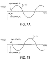
- signal V A1 is of the form:
- V A1 V D sin ⁇ t+V C cos ⁇ t
- signal V B1 is of the form:
- V B1 ⁇ V D sin ⁇ t+V C cos ⁇ t
- Voltages V A1 and V B1 are differenced by operational amplifier 425 to produce:
- V DRV corresponds to the drive motion and is used to power the drivers.
- F DRV is used as the input to a digital phase locked loop circuit 435 .
- F DRV also is supplied to a processor 440 .
- V COR is supplied to a synchronous demodulator 450 that produces an output voltage V M that is directly proportional to mass by rejecting the components of V COR that do not have the same frequency as, and are not in phase with, a gating signal Q.
- the phase locked loop circuit 435 produces Q, which is a quadrature reference signal that has the same frequency ( ⁇ ) as V DRV and is 90° out of phase with V DRV (i.e., in phase with V COR ). Accordingly, synchronous demodulator 450 rejects frequencies other than ⁇ so that V M corresponds to the amplitude of V COR at ⁇ . This amplitude is directly proportional to the mass in the conduit.
- V M is supplied to a voltage-to-frequency converter 455 that produces a square wave signal F M having a frequency that corresponds to the amplitude of V M .
- the processor 440 then divides F M by F DRV to produce a measurement of the mass flow rate.
- Digital phase locked loop circuit 435 also produces a reference signal I that is in phase with V DRV and is used to gate the synchronous demodulator 415 in the feedback loop controlling amplifier 410 .
- the summing operation at operational amplifier 445 produces zero drive component (i.e., no signal in phase with V DRV ) in the signal V COR .
- a drive component exists in V COR . This drive component is extracted by synchronous demodulator 415 and integrated by integrator 420 to generate an error voltage that corrects the gain of input amplifier 410 .
- Digital-to-analog (“D/A”) converters 515 convert digital control signals from the controller 505 to analog signals for driving the drivers 46 .
- the use of a separate drive signal for each driver has a number of advantages. For example, the system may easily switch between symmetrical and antisymmetrical drive modes for diagnostic purposes.
- the signals produced by converters 515 may be amplified by amplifiers prior to being supplied to the drivers 46 .
- a single D/A converter may be used to produce a drive signal applied to both drivers, with the drive signal being inverted prior to being provided to one of the drivers to drive the conduit 120 in the antisymmetrical mode.
- An additional temperature sensor 560 measures the temperature of the crystal oscillator 565 used by the A/D converters.
- An A/D converter 570 converts this temperature measurement to a digital signal for use by the controller 505 .
- the input/output relationship of the A/D converters varies with the operating frequency of the converters, and the operating frequency varies with the temperature of the crystal oscillator. Accordingly, the controller uses the temperature measurement to adjust the data provided by the A/D converters, or in system calibration.
- the digital controller 505 processes the digitized sensor signals produced by the A/D converters 510 according to the procedure 600 illustrated in FIG. 6 to generate the mass flow measurement and the drive signal supplied to the drivers 46 .
- the controller collects data from the sensors (step 605 ). Using this data, the controller determines the frequency of the sensor signals (step 610 ), eliminates zero offset from the sensor signals (step 615 ), and determines the amplitude (step 620 ) and phase (step 625 ) of the sensor signals. The controller uses these calculated values to generate the drive signal (step 630 ) and to generate the mass flow and other measurements (step 635 ). After generating the drive signals and measurements, the controller collects a new set of data and repeats the procedure. The steps of the procedure 600 may be performed serially or in parallel, and may be performed in varying order.
- the digitized signals from the two sensors will be referred to as signals SV 1 and SV 2 , with signal SV 1 coming from sensor 48 a and signal SV 2 coming from sensor 48 b .
- new data is generated constantly, it is assumed that calculations are based upon data corresponding to one complete cycle of both sensors. With sufficient data buffering, this condition will be true so long as the average time to process data is less than the time taken to collect the data.
- Tasks to be carried out for a cycle include deciding that the cycle has been completed, calculating the frequency of the cycle (or the frequencies of SV 1 and SV 2 ), calculating the amplitudes of SV 1 and SV 2 , and calculating the phase difference between SV 1 and SV 2 .
- start_sample_SV 1 and start_sample_SV 2 are the sampling points occurring just before the start of the cycle.
- start_offset_SV 1 or start_offset_SV 2 the position between the starting sample and the next sample at which the cycle actually begins.
- controller When the controller employs functions such as the sum (A+B) and difference (A ⁇ B), with B weighted to have the same amplitude as A, additional variables (e.g., start_sample_sum and start_offset_sum) track the start of the period for each function.
- the sum and difference functions have a phase offset halfway between SV 1 and SV 2 .
- the data structure employed to store the data from the sensors is a circular list for each sensor, with a capacity of at least twice the maximum number of samples in a cycle.
- processing may be carried out on data for a current cycle while interrupts or other techniques are used to add data for a following cycle to the lists.
- the first task in assembling data for a cycle is to determine where the cycle begins and ends.
- the beginning of the cycle may be identified as the end of the previous cycle.
- the cycles overlap by 180° the beginning of the cycle may be identified as the midpoint of the previous cycle, or as the endpoint of the cycle preceding the previous cycle.
- the end of the cycle may be first estimated based on the parameters of the previous cycle and under the assumption that the parameters will not change by more than a predetermined amount from cycle to cycle. For example, five percent may be used as the maximum permitted change from the last cycle's value, which is reasonable since, at sampling rates of 55 kHz, repeated increases or decreases of five percent in amplitude or frequency over consecutive cycles would result in changes of close to 5,000 percent in one second.
- a conservative estimate for the upper limit on the end of the cycle for signal SV 1 may be determined as: end_sample ⁇ _SV1 ⁇ start_sample ⁇ _SV1 + 365 360 * sample_rate est_freq * 0.95
- start_sample_SV 1 is the first sample of sv 1 _in
- sample_rate is the sampling rate
- est_freq is the frequency from the previous cycle.
- the upper limit on the end of the cycle for signal SV 2 (end_sample_SV 2 ) may be determined similarly.
- a cycle may not be worth processing when, for example, the conduit has stalled or the sensor waveforms are severely distorted. Processing only suitable cycles provides considerable reductions in computation.
- One way to determine cycle suitability is to examine certain points of a cycle to confirm expected behavior.
- the amplitudes and frequency of the last cycle give useful starting estimates of the corresponding values for the current cycle. Using these values, the points corresponding to 30°, 150°, 210° and 330° of the cycle may be examined. If the amplitude and frequency were to match exactly the amplitude and frequency for the previous cycle, these points should have values corresponding to est_amp/2, est_amp/2, ⁇ est_amp/2, and ⁇ est_amp/2, respectively, where est_amp is the estimated amplitude of a signal (i.e., the amplitude from the previous cycle).
- the inequalities for the other points have the same form, with the degree offset term (x/360) and the sign of the est_amp_SV 1 term having appropriate values. These inequalities can be used to check that the conduit has vibrated in a reasonable manner.
- start min(start_sample — SV 1 , start_sample — SV 2 ),
- end max(end_sample — SV 1 , end_sample — SV 2 ).
- Error sources associated with this curve fitting technique are random noise, zero offset, and deviation from a true quadratic. Curve fitting is highly sensitive to the level of random noise. Zero offset in the sensor voltage increases the amplitude of noise in the sine-squared function, and illustrates the importance of zero offset elimination (discussed below). Moving away from the minimum, the square of even a pure sine wave is not entirely quadratic. The most significant extra term is of fourth order. By contrast, the most significant extra term for linear interpolation is of third order.
- Degrees of freedom associated with this curve fitting technique are related to how many, and which, data points are used.
- the minimum is three, but more may be used (at greater computational expense) by using least-squares fitting. Such a fit is less susceptible to random noise.
- FIG. 8A illustrates that a quadratic approximation is good up to some 20° away from the minimum point. Using data points further away from the minimum will reduce the influence of random noise, but will increase the errors due to the non-quadratic terms (i.e., fourth order and higher) in the sine-squared function.
- the controller then generates a first estimate of end_point (step 910 ).
- the controller generates this estimate by calculating an estimated zero-crossing point based on the estimated frequency from the previous cycle and searching around the estimated crossing point (forwards and backwards) to find the nearest true crossing point (i.e., the occurrence of consecutive samples with different signs).
- the controller then sets end_point equal to the sample point having the smaller magnitude of the samples surrounding the true crossing point.
- the controller sets n, the number of points for curve fitting (step 915 ).
- the controller sets n equal to 5 for a sample rate of 11 kHz, and to 21 for a sample rate of 44 kHz.
- the controller then sets iteration_count to 0 (step 920 ) and increments iteration_count (step 925 ) to begin the iterative portion of the procedure.
- the procedure 900 causes the controller to make three attempts to home in on end_point, using smaller step_lengths in each attempt. If the resulting minimum for any attempt falls outside of the points used to fit the curve (i.e., there has been extrapolation rather than interpolation), this indicates that either the previous or new estimate is poor, and that a reduction in step size is unwarranted.
- the procedure 900 may be applied to at least three different sine waves produced by the sensors. These include signals SV 1 and SV 2 and the weighted sum of the two. Moreover, assuming that zero offset is eliminated, the frequency estimates produced for these signals are independent. This is clearly true for signals SV 1 and SV 2 , as the errors on each are independent. It is also true, however, for the weighted sum, as long as the mass flow and the corresponding phase difference between signals SV 1 and SV 2 are large enough for the calculation of frequency to be based on different samples in each case. When this is true, the random errors in the frequency estimates also should be independent.
- the three independent estimates of frequency can be combined to provide an improved estimate.
- This combined estimate is simply the mean of the three frequency estimates.
- An important error source in a Coriolis transmitter is zero offset in each of the sensor voltages.
- Zero offset is introduced into a sensor voltage signal by drift in the pre-amplification circuitry and the analog-to-digital converter. The zero offset effect may be worsened by slight differences in the pre-amplification gains for positive and negative voltages due to the use of differential circuitry.
- Each error source varies between transmitters, and will vary with transmitter temperature and more generally over time with component wear.
- x ( t ) a 0 /2 +a 1 cos( ⁇ t )+ a 2 cos(2 ⁇ t )+ a 3 cos(3 ⁇ t )+ . . . + b 1 sin( ⁇ t )+ b 2 sin(2 ⁇ t )+ . . .
- a non-zero offset a 0 will result in non-zero cosine terms a n .
- the amplitude of interest is the amplitude of the fundamental component (i.e., the amplitude at frequency ⁇ )
- monitoring the amplitudes of higher harmonic components i.e., at frequencies k ⁇ , where k is greater than 1) may be of value for diagnostic purposes.
- a n 2 T ⁇ ⁇ 0 T ⁇ x ⁇ ( t ) ⁇ cos ⁇ ⁇ n ⁇ ⁇ ⁇ ⁇ ⁇ t
- b n 2 T ⁇ ⁇ 0 T ⁇ x ⁇ ( t ) ⁇ sin ⁇ ⁇ n ⁇ ⁇ ⁇ ⁇ ⁇ ⁇ t .
- the controller may use a number of approaches to calculate the phase difference between signals SV 1 and SV 2 .
- phase offset is interpreted in the context of a single waveform as being the difference between the start of the cycle (i.e., the zero-crossing point) and the point of zero phase for the component of SV(t) of frequency ⁇ . Since the phase offset is an average over the entire waveform, it may be used as the phase offset from the midpoint of the cycle. Ideally, with no zero offset and constant amplitude of oscillation, the phase offset should be zero every cycle.
- the controller may determine the phase difference by comparing the phase offset of each sensor voltage over the same time period.
- the amplitude and phase may be generated using a Fourier method that eliminates the effects of higher harmonics. This method has the advantage that it does not assume that both ends of the conduits are oscillating at the same frequency.
- a frequency estimate is produced using the zero crossings to measure the time between the start and end of the cycle. If linear variation in frequency is assumed, this estimate equals the time-averaged frequency over the period.
- the controller then calculates a phase difference, assuming that the average phase and frequency of each sensor signal is representative of the entire waveform. Since these frequencies are different for SV 1 and SV 2 , the corresponding phases are scaled to the average frequency. In addition, the phases are shifted to the same starting point (i.e., the midpoint of the cycle on SV 1 ).
- phase and amplitude are not calculated over the same time-frame for the two sensors.
- the two cycle mid-points are coincident.
- a phase shift of 4° (out of 360°) means that only 99% of the samples in the SV 1 and SV 2 data sets are coincident. Far greater phase shifts may be observed under aerated conditions, which may lead to even lower rates of overlap.
- FIG. 10 illustrates a modified approach 1000 that addresses this issue.
- the controller finds the frequencies (f 1 , f 2 ) and the mid-points (m 1 , m 2 ) of the SV 1 and SV 2 data sets (d 1 , d 2 ) (step 1005 ).
- the controller calculates the frequency of SV 2 at the midpoint of SV 1 (f 2m1 ) and the frequency of SV 1 at the midpoint of SV 2 (f 1m2 ) (step 1010 ).
- the controller then calculates the starting and ending points of new data sets (d 1m2 and d 2m1 ) with mid-points m 2 and m 1 respectively, and assuming frequencies of f 1m2 and f 2m1 (step 1015 ). These end points do not necessarily coincide with zero crossing points. However, this is not a requirement for Fourier-based calculations.
- the controller also may use a difference-amplitude method that involves calculating a difference between SV 1 and SV 2 , squaring the calculated difference, and integrating the result.
- the controller synthesizes a sine wave, multiplies the sine wave by the difference between signals SV 1 and SV 2 , and integrates the result.
- the controller also may integrate the product of signals SV 1 and SV 2 , which is a sine wave having a frequency 2 f (where f is the average frequency of signals SV 1 and SV 2 ), or may square the product and integrate the result.
- ⁇ is the phase difference between the sensors.
- the controller calculates data sets for Sum and Diff from the data for SV 1 and SV 2 , and then uses one or more of the methods described above to calculate the amplitude of the signals represented by those data sets. The controller then uses the calculated amplitudes to calculate the phase difference, ⁇ .
- the calculation of phase is particularly dependent upon the accuracy of previous calculations (i.e., the calculation of the frequencies and amplitudes of SV 1 and SV 2 ).
- the controller may use multiple methods to provide separate (if not entirely independent) estimates of the phase, which may be combined to give an improved estimate.
- the Q of the conduit is high enough that the conduit will resonate only at certain discrete frequencies.
- the lowest resonant frequency for some conduits is between 65 Hz and 95 Hz, depending on the density of the process fluid, and irrespective of the drive frequency.
- pure sine waves having phases and frequencies determined as described above may be synthesized and sent to the drivers.
- This approach offers the advantage of eliminating undesirable high frequency components, such as harmonics of the resonant frequency.
- This approach also permits compensation for time delays introduced by the analog-to-digital converters, processing, and digital-to-analog converters to ensure that the phase of the drive signal corresponds to the mid-point of the phases of the sensor signals. This compensation may be provided by determining the time delay of the system components and introducing a phase shift corresponding to the time delay.
- Another approach to driving the conduit is to use square wave pulses. This is another synthesis method, with fixed (positive and negative) direct current sources being switched on and off at timed intervals to provide the required energy. The switching is synchronized with the sensor voltage phase.
- this approach does not require digital-to-analog converters.
- the amplitude of vibration of the conduit should rapidly achieve a desired value at startup, so as to quickly provide the measurement function, but should do so without significant overshoot, which may damage the meter.
- the desired rapid startup may be achieved by setting a very high gain so that the presence of random noise and the high Q of the conduit are sufficient to initiate motion of the conduit.
- high gain and positive feedback are used to initiate motion of the conduit.
- synthesis methods also may be used to initiate conduit motion when high gain is unable to do so. For example, if the DC voltage offset of the sensor voltages is significantly larger than random noise, the application of a high gain will not induce oscillatory motion. This condition is shown in FIGS. 11A-11D, in which a high gain is applied at approximately 0.3 seconds. As shown in FIGS. 11A and 11B, application of the high gain causes one of the drive signals to assume a large positive value (FIG. 11A) and the other to assume a large negative value (FIG. 11 B). The magnitudes of the drive signals vary with noise in the sensor signals (FIGS. 11 C and 11 D). However, the amplified noise is insufficient to vary the sign of the drive signals so as to induce oscillation.
- FIGS. 12A-12D illustrate that imposition of a square wave over several cycles can reliably cause a rapid startup of oscillation. Oscillation of a conduit having a two inch diameter may be established in approximately two seconds. The establishment of conduit oscillation is indicated by the reduction in the amplitude of the drive signals, as shown in FIGS. 12A and 12B.
- FIGS. 13A-13D illustrate that oscillation of a one inch conduit may be established in approximately half a second.
- a square wave also may be used during operation to correct conduit oscillation problems. For example, in some circumstances, flow meter conduits have been known to begin oscillating at harmonics of the resonant frequency of the conduit, such as frequencies on the order of 1.5 kHz. When such high frequency oscillations are detected, a square wave having a more desirable frequency may be used to return the conduit oscillation to the resonant frequency.
- the controller digitally generates the mass flow measurement in a manner similar to the approach used by the analog controller.
- the controller also may generate other measurements, such as density.
- T c is a calibration temperature
- MF 1 -MF 3 are calibration constants calculated during a calibration procedure
- noneu_mf is the mass flow in non-engineering units.
- the controller calculates the density based on the frequency of oscillation of the conduit and the process temperature:
- D 1 -D 4 are calibration constants generated during a calibration procedure.
- the basic technique may be expressed as: ⁇ t n t n + 2 ⁇ y ⁇ ⁇ t ⁇ h 3 ⁇ ( y n + 4 ⁇ y n + 1 + y n + 2 ) ,
- t k is the time at sample k
- y k is the corresponding function value
- h is the step length.
- This rule can be applied repeatedly to any data vector with an odd number of data points (i.e., three or more points), and is equivalent to fitting and integrating a cubic spline to the data points. If the number of data points happens to be even, then the so-called 3 ⁇ 8ths rule can be applied at one end of the interval: ⁇ t n t n + 3 ⁇ y ⁇ ⁇ t ⁇ 3 ⁇ h 8 ⁇ ( y n + 3 ⁇ y n + 1 + 3 ⁇ y n + 2 + y n + 3 ) .
- the controller generates an initial estimate of the nominal operating frequency of the system (step 1405 ).
- the controller attempts to measure the deviation of the frequency of a signal x[k] (e.g., SV 1 ) from this nominal frequency:
- A is the amplitude of the sine wave portion of the signal
- ⁇ 0 is the nominal frequency (e.g., 88 Hz)
- ⁇ is the deviation from the nominal frequency
- h is the sampling interval
- ⁇ is the phase shift
- ⁇ (k) corresponds to the added noise and harmonics.
- the controller synthesizes two signals that oscillate at the nominal frequency (step 1410 ).
- the signals are phase shifted by 0 and ⁇ /2 and have amplitude of unity.
- the controller multiplies each of these signals by the original signal to produce signals y 1 and y 2 (step 1415 ):
- y 1 and y 2 are high frequency (e.g., 176 Hz) components and the second terms are low frequency (e.g., 0 Hz) components.
- the controller then eliminates the high frequency components using a low pass filter (step 1420 ):
- y 1 ′ A 2 ⁇ sin ⁇ ( ⁇ ⁇ ⁇ ⁇ ⁇ ⁇ kh + ⁇ ) + ⁇ 1 ⁇ [ k ]
- y 1 ′ A 2 ⁇ cos ⁇ ( ⁇ ⁇ ⁇ ⁇ ⁇ ⁇ kh + ⁇ ) + ⁇ 2 ⁇ [ k ] ,
- ⁇ 1 [k] and ⁇ 2 [k] represent the filtered noise from the original signals.
- the controller combines these signals to produce u[k] (step 1425 ):
- u 1 [k] represents the real component of u[k]
- u 2 [k] represents the imaginary component
- the controller then adds the frequency deviation to the nominal frequency (step 1435 ) to give the actual frequency:
- the controller also uses the real and imaginary components of u[k] to determine the amplitude of the original signal. In particular, the controller determines the amplitude as (step 1440 ):
- phase difference 1 2 ⁇ arcsin ⁇ 8 ⁇ v ′ A 2 .
- This procedure relies on the accuracy with which the operating frequency is initially estimated, as the procedure measures only the deviation from this frequency. If a good estimate is given, a very narrow filter can be used, which makes the procedure very accurate. For typical flowmeters, the operating frequencies are around 95 Hz (empty) and 82 Hz (full). A first approximation of half range (88 Hz) is used, which allows a low-pass filter cut-off of 13 Hz. Care must be taken in selecting the cut-off frequency as a very small cut-off frequency can attenuate the amplitude of the sine wave.
- the accuracy of measurement also depends on the filtering characteristics employed.
- the attenuation of the filter in the dead-band determines the amount of harmonics rejection, while a smaller cutoff frequency improves the noise rejection.
- FIGS. 15A and 15B illustrate a meter 1500 having a controller 1505 that uses another technique to generate the signals supplied to the drivers.
- Analog-to-digital converters 1510 digitize signals from the sensors 48 and provide the digitized signals to the controller 1505 .
- the controller 1505 uses the digitized signals to calculate gains for each driver, with the gains being suitable for generating desired oscillations in the conduit. The gains may be either positive or negative.
- the controller 1505 then supplies the gains to multiplying digital-to-analog converters 1515 .
- two or more multiplying digital-to-analog converters arranged in series may be used to implement a single, more sensitive multiplying digital-to-analog converter.
- the controller 1505 also generates drive signals using the digitized sensor signals.
- the controller 1505 provides these drive signals to digital-to-analog converters 1520 that convert the signals to analog signals that are supplied to the multiplying digital-to-analog converters 1515 .
- FIG. 15B illustrates the control approach in more detail.
- the digitized sensor signals are provided to an amplitude detector 1550 , which determines a measure, a(t), of the amplitude of motion of the conduit using, for example, the technique described above.
- a summer 1555 then uses the amplitude a(t) and a desired amplitude ao to calculate an error e(t) as:
- the error e(t) is used by a proportional-integral (“PI”) control block 1560 to generate a gain K 0 (t). This gain is multiplied by the difference of the sensor signals to generate the drive signal.
- the PI control block permits high speed response to changing conditions.
- the amplitude detector 1550 , summer 1555 , and PI control block 1560 may be implemented as software processed by the controller 1505 , or as separate circuitry.
- the meter 1500 operates according to the procedure 1600 illustrated in FIG. 16 .
- the controller receives digitized data from the sensors (step 1605 ).
- the procedure 1600 includes three parallel branches: a measurement branch 1610 , a drive signal generation branch 1615 , and a gain generation branch 1620 .
- the digitized sensor data is used to generate measurements of amplitude, frequency, and phase, as described above (step 1625 ). These measurements then are used to calculate the mass flow rate (step 1630 ) and other process variables.
- the controller 1505 implements the measurement branch 1610 .
- the digitized signals from the two sensors are differenced to generate the signal (step 1635 ) that is multiplied by the gain to produce the drive signal.
- this differencing operation is performed by the controller 1505 .
- the differencing operation produces a weighted difference that accounts for amplitude differences between the sensor signals.
- the objective of the PI control block is to sustain in the conduit pure sinusoidal oscillations having an amplitude a 0 .
- the behavior of the conduit may be modeled as a simple mass-spring system that may be expressed as:
- a two-term PI control block that gives zero steady-state error may be expressed as:
- K 0 ( t ) K p e ( t )+ K i ⁇ 0 1 e ( t ) dt,
- a linear model of the behavior of the oscillation amplitude may be derived by assuming that x(t) equals A ⁇ j ⁇ t , which results in:
- A(t) also may be expressed as: A .
- A - ⁇ ⁇ ⁇ ⁇ n + k ⁇ ⁇ K 0 2 ⁇ ⁇ t .
- ⁇ n is a “load disturbance” that needs to be eliminated by the controller (i.e., kK o /2 must equal ⁇ n for a(t) to be constant). For zero steady-state error this implies that the outer-loop controller must have an integrator (or very large gain).
- an appropriate PI controller, C(s) may be assumed to be K p (1+1/sT i ), where T i is a constant. The proportional term is required for stability.
- p 2 is a second-order polynomial.
- the signal p(t) increases and then decays to zero so that e(t), which is proportional to p′, must change sign, implying overshoot in a(t).
- T i is the known controller parameter.
- real controller poles should provide overshoot-free step responses. This feature is useful as there may be physical constraints on overshoot (e.g., mechanical interference or overstressing of components).
- A is the amplitude of an oscillation which might be growing or decaying and hence cannot in general be measured without taking into account the underlying sinusoid.
- There are several possible methods for measuring A in addition to those discussed above. Some are more suitable for use in quasi-steady conditions.
- the AM detector is the simplest approach. Moreover, it does not presume that there are oscillations of any particular frequency, and hence is usable during startup conditions. It suffers from a disadvantage that there is a leakage of harmonics into the inner loop which will affect the spectrum of the resultant oscillations.
- the filter adds extra dynamics into the outer loop such that compromises need to be made between speed of response and spectral purity. In particular, an effect of the filter is to constrain the choice of the best T i .
- zero offset may be introduced into a sensor voltage signal by drift in the pre-amplification circuitry and by the analog-to-digital converter. Slight differences in the pre-amplification gains for positive and negative voltages due to the use of differential circuitry may worsen the zero offset effect. The errors vary between transmitters, and with transmitter temperature and component wear.
- Audio quality (i.e., relatively low cost) analog-to-digital converters may be employed for economic reasons. These devices are not designed with DC offset and amplitude stability as high priorities.
- FIGS. 19A-19D show how offset and positive and negative gains vary with chip operating temperature for one such converter (the AD1879 converter). The repeatability of the illustrated trends is poor, and even allowing for temperature compensation based on the trends, residual zero offset and positive/negative gain mismatch remain.
- FIGS. 20A-20C Each graph shows the calculated phase offset as measured by the digital transmitter when the true phase offset is zero (i.e., at zero flow).
- FIG. 20A shows phase calculated based on whole cycles starting with positive zero-crossings.
- the mean value is 0.00627 degrees.
- FIG. 20B shows phase calculated starting with negative zero-crossings.
- the mean value is 0.0109 degrees.
- FIG. 20C shows phase calculated every half-cycle.
- FIG. 20C interleaves the data from FIGS. 20A and 20B.
- the average phase ( ⁇ 0.00234) is closer to zero than in FIGS. 20A and 20B, but the standard deviation of the signal is about six times higher.
- phase measurement techniques such as those based on Fourier methods, are immune to DC offset. However, it is desirable to eliminate zero offset even when those techniques are used, since data is processed in whole-cycle packets delineated by zero crossing points. This allows simpler analysis of the effects of, for example, amplitude modulation on apparent phase and frequency. In addition, gain mismatch between positive and negative voltages will introduce errors into any measurement technique.
- FIGS. 21A and 21B illustrate the long term drift in phase with zero flow. Each point represents an average over one minute of live data.
- FIG. 21A shows the average phase
- FIG. 21B shows the standard deviation in phase. Over several hours, the drift is significant. Thus, even if the meter were zeroed every day, which in many applications would be considered an excessive maintenance requirement, there would still be considerable phase drift.
- a technique for dealing with voltage offset and gain mismatch uses the computational capabilities of the digital transmitter and does not require a zero flow condition.
- the technique uses a set of calculations each cycle which, when averaged over a reasonable period (e.g., 10,000 cycles), and excluding regions of major change (e.g., set point change, onset of aeration), converge on the desired zero offset and gain mismatch compensations.
- the desired waveform for a sensor voltage SV(t) is of the form:
- ⁇ G represents the gain mismatch
- the technique assumes that the amplitudes A i and the frequency ⁇ are constant. This is justified because estimates of Z o and ⁇ G are based on averages taken over many cycles (e.g., 10,000 interleaved cycles occurring in about 1 minute of operation).
- the controller tests for the presence of significant changes in frequency and amplitude to ensure the validity of the analysis.
- the presence of the higher harmonics leads to the use of Fourier techniques for extracting phase and amplitude information for specific harmonics. This entails integrating SV(t) and multiplying by a modulating sine or cosine function.
- the subscript 1 indicates the first harmonic
- N and P indicate, respectively, the negative or positive half cycle
- s and c indicate, respectively, whether a sine or a cosine modulating function has been used.
- the mid-zero crossing point and hence the corresponding integral limits, should be given by ⁇ / ⁇ t Zo , rather than ⁇ / ⁇ +t Zo .
- the use of the exact mid-point rather than the exact zero crossing point leads to an easier analysis, and better numerical behavior (due principally to errors in the location of the zero crossing point).
- the only error introduced by using the exact mid-point is that a small section of each of the above integrals is multiplied by the wrong gain (1 instead of 1+ ⁇ G and vice versa). However, these errors are of order Z o 2 ⁇ G and are considered negligible.
- Useful related functions including the sum, difference, and ratio of the integrals and their estimates may be determined.
- the sum of the integrals may be expressed as:
- Diff 1 ⁇ s_est A 1 ⁇ ⁇ ⁇ G + 4 ⁇ ⁇ ⁇ Z 0 ⁇ ⁇ ( 2 + ⁇ G ) ⁇ [ 1 + 2 3 ⁇ ⁇ A 2 A 1 + 4 15 ⁇ ⁇ A 4 A 1 ] .
- I 1 ⁇ Pc 2 ⁇ ⁇ ⁇ ⁇ ⁇ t z 0 ⁇ ⁇ + t z 0 ⁇ ( SV ⁇ ( t ) + Z 0 ) ⁇ cos ⁇ [ ⁇ ⁇ ( t - t z 0 ) ] ⁇ ⁇ ⁇ t
- I 1 ⁇ Nc 2 ⁇ ⁇ ⁇ ⁇ ( 1 + ⁇ G ) ⁇ ⁇ ⁇ + t z 0 2 ⁇ ⁇ ⁇ + t z 0 ⁇ ( SV ⁇ ( t ) + Z 0 ) ⁇ cos ⁇ [ ⁇ ⁇ ( t - t z 0 ) ] ⁇ ⁇ ⁇ t ,
- I 2 ⁇ Ps_est A 2 + 8 15 ⁇ ⁇ ⁇ Z 0 ⁇ [ - 5 + 9 ⁇ A 3 A 1 ]
- I 2 ⁇ Ps_est ( 1 + ⁇ G ) ⁇ [ A 2 - 8 15 ⁇ ⁇ ⁇ Z 0 ⁇ [ - 5 + 9 ⁇ A 3 A 1 ] ]
- I 2 ⁇ Ps_est ( 1 + ⁇ G ) ⁇ [ A 2 - 8 15 ⁇ ⁇ ⁇ Z 0 ⁇ [ - 5 + 9 ⁇ A 3 A 1 ] ] ,
- the integrals can be calculated numerically every cycle. As discussed below, the equations estimating the values of the integrals in terms of various amplitudes and the zero offset and gain values are rearranged to give estimates of the zero offset and gain terms based on the calculated integrals.
- the accuracy of the estimation equations may be illustrated with an example. For each basic integral, three values are provided: the “true” value of the integral (calculated within Mathcad using Romberg integration), the value using the estimation equation, and the value calculated by the digital transmitter operating in simulation mode, using Simpson's method with end correction.
- I 1Ps 2 ⁇ ⁇ ⁇ ⁇ ⁇ t z 0 ⁇ ⁇ + t z 0 ⁇ ( SV ⁇ ( t ) + Z 0 ) ⁇ sin [ ⁇ ⁇ ⁇ ( t - t z 0 ) ] ⁇ ⁇ ⁇ t
- the first order estimates for the integrals define a series of non-linear equations in terms of the amplitudes of the harmonics, the zero offset, and the gain mismatch. As the equations are non-linear, an exact solution is not readily available. However, an approximation followed by corrective iterations provides reasonable convergence with limited computational overhead.
- the zero offset compensation technique may be implemented according to the procedure 2200 illustrated in FIG. 22 .
- the controller calculates the integrals I 1Ps , I 1Ns , I 1Pc , I 1Nc , I 2Ps , I 2Ns and related functions sum 1s , ration 1s , sum 1c and sum 2s (step 2205 ). This requires minimal additional calculation beyond the conventional Fourier calculations used to determine frequency, amplitude and phase.
- the controller checks on the slope of the sensor voltage amplitude A 1 , using a conventional rate-of-change estimation technique (step 2210 ). If the amplitude is constant (step 2215 ), then the controller proceeds with calculations for zero offset and gain mismatch. This check may be extended to test for frequency stability.
- the controller To perform the calculations, the controller generates average values for the functions (e.g., sum 1s ) over the last 10,000 cycles. The controller then makes a first estimation of zero offset and gain mismatch (step 2225 ):
- the controller calculates an inverse gain factor (k) and amplitude factor (amp_factor) (step 2230 ):
- amp_factor 1+50/75*Sum 2s /Sum 1s
- the controller uses the inverse gain factor and amplitude factor to make a first estimation of the amplitudes (step 2235 ):
- the controller then improves the estimate by the following calculations, iterating as required (step 2240 ):
- ⁇ G [1+8/ ⁇ * x 1 /A 1 *amp_factor]/Ratio 1s ⁇ 1.0
- a 2 k*[Sum 2s /2 ⁇ 4/(15* ⁇ )* x 1 *x 2 *(5 ⁇ 4.5* A 2 )].
- the controller uses standard techniques to test for convergence of the values of Z o and ⁇ G . In practice the corrections are small after the first iteration, and experience suggests that three iterations are adequate.
- the controller adjusts the raw data to eliminate Z o and ⁇ G (step 2245 ).
- the controller then repeats the procedure.
- the functions i.e., sum 1s
- these subsequent values for Z o and ⁇ G reflect residual zero offset and gain mismatch, and are summed with previously generated values to produce the actual zero offset and gain mismatch.
- the controller generates adjustment parameters (e.g., S 1 _off and S 2 _off) that are used in converting the analog signals from the sensors to digital data.
- FIGS. 23A-23C, 24 A and 24 B show results obtained using the procedure 2200 .
- the short-term behavior is illustrated in FIGS. 23A-23C. This shows consecutive phase estimates obtained five minutes after startup to allow time for the procedure to begin affecting the output. Phase is shown based on positive zero-crossings, negative zero-crossings, and both.
- the difference between the positive and negative mean values has been reduced by a factor of 20, with a corresponding reduction in mean zero offset in the interleaved data set.
- the corresponding standard deviation has been reduced by a factor of approximately 6.
- noise becomes more significant as the measurement calculation rate increases.
- Other noise terms may be introduced by physical factors, such as flowtube dynamics, dynamic non-linearities (e.g. flowtube stiffness varying with amplitude), or the dynamic consequences of the sensor voltages providing velocity data rather than absolute position data.
- the described techniques exploit the high precision of the digital meter to monitor and compensate for dynamic conduit behavior to reduce noise so as to provide more precise measurements of process variables such as mass flow and density. This is achieved by monitoring and compensating for such effects as the rates of change of frequency, phase and amplitude, flowtube dynamics, and dynamic physical non-idealities. A phase difference calculation which does not assume the same frequency on each side has already been described above. Other compensation techniques are described below.
- phase noise in a Coriolis flowmeter may be attributed to flowtube dynamics (sometimes referred to as “ringing”), rather than to process conditions being measured.
- the application of a dynamic model can reduce phase noise by a factor of 4 to 10, leading to significantly improved flow measurement performance.
- a single model is effective for all flow rates and amplitudes of oscillation. Generally, computational requirements are negligible.
- phase is conventionally defined in terms of the difference between the sensor voltages.
- phase for the individual sensor may be defined in terms of the difference between the midpoint of the cycle and the average 180° phase point.
- cycle n is from time 0 to 2 ⁇ / ⁇ .
- the average values of amplitude, frequency and phase equal the instantaneous values at the mid-point, ⁇ / ⁇ , which is also the starting point for cycle n+1, which is from time ⁇ / ⁇ to 3 ⁇ / ⁇ .
- ⁇ / ⁇ the instantaneous values at the mid-point
- cycle n+1 which is from time ⁇ / ⁇ to 3 ⁇ / ⁇ .
- these timings are approximate, since ⁇ also varies with time.
- the controller accounts for dynamic effects according to the procedure 2600 illustrated in FIG. 26 .
- the controller produces a frequency estimate (step 2605 ) by using the zero crossings to measure the time between the start and end of the cycle, as described above. Assuming that frequency varies linearly, this estimate equals the time-averaged frequency over the period.
- the controller uses the estimated frequency to generate a first estimate of amplitude and phase using the Fourier method described above (step 2610 ). As noted above, this method eliminates the effects of higher harmonics.
- the controller then calculates a phase difference (step 2615 ).
- a phase difference (step 2615 )
- the analysis assumes that the average phase and frequency of each sensor signal is representative of the entire waveform. Since these frequencies are different for SV 1 and SV 2 , the corresponding phases are scaled to the average frequency. In addition, the phases are shifted to the same starting point (i.e., the midpoint of the cycle on SV 1 ). After scaling, they are subtracted to provide the phase difference.
- a revised estimate of the rate of change can be calculated after amplitude correction has been applied (as described below). This results in iteration to convergence for the best values of amplitude and rate of change.
- ⁇ (t) is the phase delay caused by the feedback effect.
- the mechanical Q of the oscillating conduit is typically on the order of 1000, which implies small deviations in amplitude and phase.
- ⁇ (t) is given by: ⁇ ⁇ ( t ) ⁇ - A . ⁇ ( t ) 2 ⁇ ⁇ 0 ⁇ A ⁇ ( t ) ⁇
- the expression for the velocity offset phase delay may be simplified to: ⁇ ⁇ ( t ) ⁇ A . ⁇ ( t ) ⁇ 0 ⁇ A ⁇ ( t ) ⁇
- the actual frequency of oscillation may be distinguished from the natural frequency of oscillation. Though the former is observed, the latter is useful for density calculations. Over any reasonable length of time, and assuming adequate amplitude control, the averages of these two frequencies are the same (because the average rate of change of amplitude must be zero). However, for improved instantaneous density measurement, it is desirable to compensate the actual frequency of oscillation for dynamic effects to obtain the natural frequency. This is particularly useful in dealing with aerated fluids for which the instantaneous density can vary rapidly with time.
- error_sum 0 - 1 8 ⁇ ⁇ 2 ⁇ ( A . 0 A 0 + A . 1 A 1 ) ⁇
- FIGS. 27A-32B illustrate how application of the procedure 2600 improves the estimate of the natural frequency, and hence the process density, for real data from a meter having a one inch diameter conduit.
- Each of the figures shows 10,000 samples, which are collected in just over 1 minute.
- FIGS. 27A and 27B show amplitude and frequency data from SV 1 , taken when random changes to the amplitude set-point have been applied. Since the conduit is full of water and there is no flow, the natural frequency is constant. However, the observed frequency varies considerably in response to changes in amplitude. The mean frequency value is 81.41 Hz, with a standard deviation of 0.057 Hz.
- FIGS. 28A and 28B show, respectively, the variation in frequency from the mean value, and the correction term generated using the procedure 2600 .
- the gross deviations are extremely well matched. However, there is additional variance in frequency which is not attributable to amplitude variation.
- Another important feature illustrated by FIG. 28B is that the average is close to zero as a result of the proper initialization of the error term, as described above.
- FIGS. 29A and 92B compare the raw frequency data (FIG. 29A) with the results of applying the correction function (FIG. 29 B). There has been a negligible shift in the mean frequency, while the standard deviation has been reduced by a factor of 4.4. From FIG. 29B, it is apparent that there is residual structure in the corrected frequency data. It is expected that further analysis, based on the change in phase across a cycle and its impact on the observed frequency, will yield further noise reductions.
- FIGS. 30A and 30B show the corresponding effect on the average frequency, which is the mean of the instantaneous sensor voltage frequencies. Since the mean frequency is used to calculate the density of the process fluid, the noise reduction (here by a factor of 5.2) will be propagated into the calculation of density.
- FIGS. 31A and 31B illustrate the raw and corrected average frequency for a 2′′ diameter conduit subject to a random amplitude set-point.
- the 2′′ flowtube exhibits less frequency variation that the 1′′, for both raw and corrected data.
- the noise reduction factor is 4.0.
- the controller next compensates the phase measurement to account for amplitude modulation assuming the phase calculation provided above (step 2630 ).
- the Fourier calculations of phase described above assume that the amplitude of oscillation is constant throughout the cycle of data on which the calculations take place. This section describes a correction which assumes a linear variation in amplitude over the cycle of data.
- I 1 A 1 ⁇ ( 1 + ⁇ ⁇ ⁇ ⁇ A )
- I 2 A 1 ⁇ 1 2 ⁇ ⁇ ⁇ ⁇ A .
- Simulations have been carried out using the digital transmitter, including the simulation of higher harmonics and amplitude modulation.
- Theory suggests a phase offset of ⁇ 0.02706 degrees. In simulation over 1000 cycles, the average offset is ⁇ 0.02714 degrees, with a standard deviation of only 2.17e ⁇ 6 .
- the difference between simulation and theory (approx 0.3% of the simulation error) is attributable to the model's assumption of a linear variation in amplitude over each cycle, while the simulation generates an exponential change in amplitude.
- FIGS. 33A-34B give examples of how this correction improves real flowmeter data.
- FIG. 33A shows raw phase data from SV 1 , collected from a 1′′ diameter conduit, with low flow assumed to be reasonably constant.
- FIG. 33B shows the correction factor calculated using the formula described above, while
- FIG. 33C shows the resulting corrected phase.
- the most apparent feature is that the correction has increased the variance of the phase signal, while still producing an overall reduction in the phase difference (i.e., SV 2 ⁇ SV 1 ) standard deviation by a factor of 1.26, as shown in FIGS. 34A and 34B.
- the improved performance results because this correction improves the correlation between the two phases, leading to reduced variation in the phase difference.
- the technique works equally well in other flow conditions and on other conduit sizes.
- phase measurement calculation is also affected by the velocity effect.
- ⁇ SV is an estimate of the rate of change of SV, scaled by its absolute value, and is also referred to as the proportional rate of change of SV.
- FIGS. 36A-36L Each graph shows three phase difference measurements calculated simultaneously in real time by the digital Coriolis transmitter operating on a one inch conduit.
- the middle band 3600 shows phase data calculated using the simple time-difference technique.
- the outermost band 3605 shows phase data calculated using the Fourier-based technique described above.
- the innermost band of data 3610 shows the same Fourier data after the application of the sensor-level noise reduction techniques. As can be seen, substantial noise reduction occurs in each case, as indicated by the standard deviation values presented on each graph.
- a dynamic model may be incorporated in two basic stages.
- the model is created using the techniques of system identification.
- the flowtube is “stimulated” to manifest its dynamics, while the true mass flow and density values are kept constant.
- the response of the flowtube is measured and used in generating the dynamic model.
- the model is applied to normal flow data. Predictions of the effects of flowtube dynamics are made for both phase and frequency. The predictions then are subtracted from the observed data to leave the residual phase and frequency, which should be due to the process alone.
- System identification begins with a flowtube full of water, with no flow.
- the amplitude of oscillation which normally is kept constant, is allowed to vary by assigning a random setpoint between 0.05 V and 0.3 V, where 0.3 V is the usual value.
- the resulting sensor voltages are shown in FIG. 37A, while FIGS. 37B and 37C show, respectively, the corresponding calculated phase and frequency values. These values are calculated once per cycle. Both phase and frequency show a high degree of “structure.” Since the phase and frequency corresponding to mass flow are constant, this structure is likely to be related to flowtube dynamics. Observable variables that will predict this structure when the true phase and frequency are not known to be constant may be expressed as set forth below.
- This expression may be used to determine ⁇ SV 1 and ⁇ SV 2 .
- the phase of the flowtube is related to ⁇ , which is defined as ⁇ SV 1 ⁇ SV 2
- the frequency is related to ⁇ + , which is defined as ⁇ SV 1 + ⁇ SV 2 .
- Some correction for flowtube dynamics may be obtained by subtracting a multiple of the appropriate prediction function from the phase and/or the frequency. Improved results may be obtained using a model of the form:
- y(k) is the output (i.e., phase or frequency) and u is the prediction function (i.e., ⁇ ⁇ or ⁇ + ).
- u is the prediction function (i.e., ⁇ ⁇ or ⁇ + ).
- the technique of system identification suggests values for the orders n and m, and the coefficients a i and b j , of what are in effect polynomials in time.
- the value of y(k) can be calculated every cycle and subtracted from the observed phase or frequency to get the residual process value.
- the digital flowmeter offers very good precision over a long period of time. For example, when totalizing a batch of 200 kg, the device readily achieves a repeatability of less that 0.03%.
- the purpose of the dynamic modeling is to improve the dynamic precision.
- raw and compensated values should have similar mean values, but reductions in “variance” or “standard deviation.”
- FIGS. 38A and 39A show raw and corrected frequency values.
- the mean values are similar, but the standard deviation has been reduced by a factor of 3.25. Though the gross deviations in frequency have been eliminated, significant “structure” remains in the residual noise. This structure appears to be unrelated to the ⁇ + function.
- FIGS. 38C and 39C show the effects of correction under these conditions. As shown, the standard deviation is reduced by a factor of 31. This more effective model is used in the following discussions.
- phase values are plotted at 82 Hz or thereabouts. The reported standard deviation would be roughly 1 ⁇ 3 of the values shown when averaged to 10 Hz, and ⁇ fraction (1/9) ⁇ when averages to 1 Hz. For reference, on a one inch flow tube, one degree of phase difference corresponds to about 1 kg/s flow rate.
- FIGS. 38D and 39D show the correction applied to a full flowtube with zero flow, just after startup.
- the ring-down effect characteristic of startup is clearly evident in the raw data (FIG. 38 D), but this is eliminated by the correction (FIG. 39 D), leading to a standard deviation reduction of a factor of 23 over the whole data set. Note that the corrected measurement closely resembles white noise, suggesting most flowtube dynamics have been captured.
- FIGS. 38E and 39E show the resulting correction for a “drained” flowtube. Noise is reduced by a factor of 6.5 or so. Note, however, that there appears to be some residual structure in the noise.
- the digital flowmeter provides improved performance in the presence of aeration in the conduit.
- Aeration causes energy losses in the conduit that can have a substantial negative impact on the measurements produced by a mass flowmeter and can result in stalling of the conduit.
- the digital flowmeter has substantially improved performance in the presence of aeration relative to traditional, analog flowmeters. This performance improvement may stem from the meter's ability to provide a very wide gain range, to employ negative feedback, to calculate measurements precisely at very low amplitude levels, and to compensate for dynamic effects such as rate of change of amplitude and flowtube dynamics, and also may stem from the meter's use of a precise digital amplitude control algorithm.
- the digital flowmeter detects the onset of aeration when the required driver gain rises simultaneously with a drop in apparent fluid density.
- the digital flowmeter then may directly respond to detected aeration.
- the meter monitors the presence of aeration by comparing the observed density of the material flowing through the conduit (i.e., the density measurement obtained through normal measurement techniques) to the known, nonaerated density of the material.
- the controller determines the level of aeration based on any difference between the observed and actual densities. The controller then corrects the mass flow measurement accordingly.
- the controller determines the non-aerated density of the material by monitoring the density over time periods in which aeration is not present (i.e., periods in which the density has a stable value).
- a control system to which the controller is connected may provide the non-aerated density as an initialization parameter.
- the controller uses three corrections to account for the effects of aeration: bubble effect correction, damping effect correction, and sensor imbalance correction.
- FIGS. 40A-40H illustrate the effects of the correction procedure.
- FIG. 40A illustrates the error in the phase measurement as the measured density decreases (i.e., as aeration increases) for different mass flow rates, absent aeration correction. As shown, the phase error is negative and has a magnitude that increases with increasing aeration. FIG. 40B illustrates that the resulting mass flow error is also negative. It also is significant to note that the digital flowmeter operates at high levels of aeration. By contrast, as indicated by the horizontal bar 4000 , traditional analog meters tend to stall in the presence of low levels of aeration.
- a stall occurs when the flowmeter is unable to provide a sufficiently large driver gain to allow high drive current at low amplitudes of oscillation. If the level of damping requires a higher driver gain than can be delivered by the flowtube in order to maintain oscillation at a certain amplitude, then insufficient drive energy is supplied to the conduit. This results in a drop in amplitude of oscillation, which in turn leads to even less drive energy supplied due to the maximum gain limit. Catastrophic collapse results, and flowtube oscillation is not possible until the damping reduces to a level at which the corresponding driver gain requirement can be supplied by the flowmeter.
- the bubble effect correction is based on the assumption that the mass flow decreases as the level of aeration, also referred to as the void fraction, increases. Without attempting to predict the actual relationship between void fraction and the bubble effect, this correction assumes, with good theoretical justification, that the effect on the observed mass flow will be the same as the effect on the observed density. Since the true fluid density is known, the bubble effect correction corrects the mass flow rate by the same proportion. This correction is a linear adjustment that is the same for all flow rates.
- FIGS. 40C and 40D illustrate, respectively. the residual phase and mass flow errors after correction for the bubble effect. As shown, the residual errors are now positive and substantially smaller in magnitude than the original errors.
- the damping factor correction accounts for damping of the conduit motion due to aeration.
- FIG. 40E illustrates the damping correction for different mass flow rates and different levels of aeration.
- FIG. 40F illustrates the residual phase error after correction for damping. As shown, the phase error is reduced substantially relative to the phase error remaining after bubble effect correction.
- the sensor balance correction is based on density differences between different ends of the conduit. As shown in FIG. 41, a pressure drop between the inlet and the outlet of the conduit results in increasing bubble sizes from the inlet to the outlet. Since material flows serially through the two loops of the conduit, the bubbles at the inlet side of the conduit (i.e., the side adjacent to the first sensor/driver pair) will be smaller than the bubbles at the outlet side of the conduit (i.e., the side adjacent to the second sensor/driver pair). This difference in bubble size results in a difference in mass and density between the two ends of the conduit. This difference is reflected in the sensor signals (SV 1 and SV 2 ). Accordingly, the sensor balance correction is based on a ratio of the two sensor signals.
- FIG. 40G illustrates the sensor balance correction for different mass flow rates and different levels of aeration.
- FIG. 40H illustrates the residual phase error after applying the sensor balance correction. At low flow rates and low levels of aeration, the phase error is improved relative to the phase error remaining after damping correction.
- correction factors also could be used.
- the phase angle of each sensor signal could be monitored.
- the average phase angle for a signal should be zero.
- the average phase angle tends to increase with increasing aeration. Accordingly, a correction factor could be generated based on the value of the average phase angle.
- Another correction factor could be based on the temperature of the conduit.
- correction factors tends to keep the mass flow errors at one percent or less. Moreover, these correction factors appear to be applicable over a wide range of flows and aeration levels.
- the digital flowmeter provides improved control of the setpoint for the amplitude of oscillation of the conduit.
- feedback control is used to maintain the amplitude of oscillation of the conduit at a fixed level corresponding to a desired peak sensor voltage (e.g., 0.3 V).
- a desired peak sensor voltage e.g., 0.3 V.
- Circumstances may arise in which it is not possible to maintain the large amplitude of oscillation due to limitations in the current that can be supplied to the drivers.
- the current is limited to 100 mA for safety purposes. This is typically 5-10 times the current needed to maintain the desired amplitude of oscillation.
- the process fluid provides significant additional damping (e.g., via two-phase flow), then the optimal amplitude may no longer be sustainable.
- a low-power flowmeter such as the two-wire meter described below, may have much less power available to drive the conduit.
- the power level may vary when the conduit is driven by capacitive discharge.
- the controller determines whether the filtered drive current exceeds a threshold level (step 4225 ). In one implementation, the threshold level is ninety five percent of the maximum available current. If the current exceeds the threshold, the controller reduces the setpoint (step 4230 ). To allow time for the meter to settle after the setpoint change, the controller then implements a pause of the procedure by setting the pause cycle count equal to an appropriate value (e.g., 100) (step 4235 ).
- an appropriate value e.g. 100
- the controller determines if it is greater than the maximum permitted setpoint (step 4260 ). If so, the controller sets the setpoint equal to the maximum permitted setpoint (step 4265 ). Otherwise, the controller sets the setpoint equal to the possible new setpoint (step 4270 ). The controller then implements a pause of the procedure by setting the pause cycle count equal to an appropriate value (step 4235 ).
- FIGS. 43A-43C illustrate operation of the setpoint adjustment procedure.
- the system starts with a setpoint of 0.3 V.
- aeration results in a drop in the apparent density of the material in the conduit (FIG. 43 A).
- Increased damping accompanying the aeration results in an increase in the drive current (FIG. 43B) and increased noise in the sensor voltage (FIG. 43 C). No changes are made at this time, since the meter is able to maintain the desired setpoint.
- the controller responds to this condition by increasing the setpoint (FIG. 43 C).
- the level of aeration decreases and the apparent density increases again at about 48 seconds of operation, and the controller responds by increasing the setpoint to 0.3 V.
- the digital flowmeter has shown remarkable performance improvements relative to traditional analog flowmeters.
- the ability of the two types of meters to accurately measure a batch of material was examined.
- the batch was fed through the appropriate flowmeter and into a tank, where the batch was then weighed.
- the analog meter provided an average offset of 500 pounds, with a repeatability of 200 pounds.
- the digital meter provided an average offset of 40 pounds, with a repeatability of two pounds, which clearly is a substantial improvement.
- the conduit and surrounding pipework were empty at the start of the batch. This is important in many batching applications where it is not practical to start the batch with the conduit full.
- the batches were finished with the flowtube full.
- Some positive offset is expected because the flowmeter is measuring the material needed to fill the pipe before the weighing tank starts to be filled. Delays in starting up, or offsets caused by aerated flow or low amplitudes of oscillation, are likely to introduce negative offsets. For real batching applications, the most important issue is the repeatability of the measurement.
- FIG. 44 illustrates the accuracy and corresponding uncertainty of the measurements produced by the two types of meters at different percentages of the meters's maximum recommended flow rate.
- the analog meter produces measurements that correspond to actual values to within 0.15% or less, compared to 0.005% or less for the digital meter.
- the offset of the analog meter is on the order of 1.5%, compared to 0.25% for the digital meter.
- the digital flowmeter may be used in a control system that includes self-validating sensors. To this end, the digital flowmeter may be implemented as a self-validating meter. Self-validating meters and other sensors are described in U.S. Pat. No. 5,570,300, entitled “SELF-VALIDATING SENSORS”, which is incorporated by reference.
- a self-validating meter provides, based on all information available to the meter, a best estimate of the value of a parameter (e.g., mass flow) being monitored. Because the best estimate is based, in part, on nonmeasurement data, the best estimate does not always conform to the value indicated by the current, possibly faulty, measurement data.
- a self-validating meter also provides information about the uncertainty and reliability of the best estimate, as well as information about the operational status of the sensor. Uncertainty information is derived from known uncertainty analyses and is provided even in the absence of faults.
- a self-validating meter provides four basic parameters: a validated measurement value (VMV), a validated uncertainty (VU), an indication (MV status) of the status under which the measurement was generated, and a device status.
- VMV is the meter's best estimate of the value of a measured parameter.
- the VU and the MV status are associated with the VMV.
- the meter produces a separate VMV, VU and MV status for each measurement.
- the device status indicates the operational status of the meter.
- the meter also may provide other information. For example, upon a request from a control system, the meter may provide detailed diagnostic information about the status of the meter. Also, when a measurement has exceeded, or is about to exceed, a predetermined limit, the meter can send an alarm signal to the control system. Different alarm levels can be used to indicate the severity with which the measurement has deviated from the predetermined value.
- VMV and VU are numeric values.
- VMV could be a temperature measurement valued at 200 degrees and VU, the uncertainty of VMV, could be 9 degrees. In this case, there is a high probability (typically 95%) that the actual temperature being measured falls within an envelope around VMV and designated by VU (i.e., from 191 degrees to 209 degrees).
- the controller generates VMV based on underlying data from the sensors.
- the controller derives a raw measurement value (RMV) that is based on the signals from the sensors.
- RMV raw measurement value
- the controller has nominal confidence in the RMV and sets the VMV equal to the RMV.
- the controller detects an abnormality in the sensor, the controller does not set the VMV equal to the RMV. Instead, the controller sets the VMV equal to a value that the controller considers to be a better estimate than the RMV of the actual parameter.
- the controller generates the VU based on a raw uncertainty signal (RU) that is the result of a dynamic uncertainty analysis of the RMV.
- RU raw uncertainty signal
- the controller performs this uncertainty analysis during each sampling period.
- Uncertainty analysis originally described in “Describing Uncertainties in Single Sample Experiments,” S. J. Kline & F. A. McClintock, Mech. Eng., 75, 3-8 (1953), has been widely applied and has achieved the status of an international standard for calibration. Essentially, an uncertainty analysis provides an indication of the “quality” of a measurement. Every measurement has an associated error, which, of course, is unknown. However, a reasonable limit on that error can often be expressed by a single uncertainty number (ANSI/ASME PTC 19.1-1985 Part 1, Measurement Uncertainty: Instruments and Apparatus).
- M is true (M true ) with a certain level of confidence (typically 95%). This uncertainty is readily expressed in a relative form as a proportion of the measurement (i.e. w M /M).
- the VU has a non-zero value even under ideal conditions (i.e., a faultless sensor operating in a controlled, laboratory environment). This is because the measurement produced by a sensor is never completely certain and there is always some potential for error.
- the controller when the controller detects no abnormalities, the controller sets the VU equal to the RU.
- the controller When the controller detects a fault that only partially affects the reliability of the RMV, the controller typically performs a new uncertainty analysis that accounts for effects of the fault and sets the VU equal to the results of this analysis.
- the controller sets the VU to a value based on past performance when the controller determines that the RMV bears no relation to the actual measured value.
- the MV status provides information about how they were calculated.
- the controller produces the VMV and the VU under all conditions—even when the sensors are inoperative.
- the control system needs to know whether VMV and VU are based on “live” or historical data. For example, if the control system were using VMV and VU in feedback control and the sensors were inoperative, the control system would need to know that VMV and VU were based on past performance.
- the MV status is based on the expected persistence of any abnormal condition and on the confidence of the controller in the RMV.
- the four primary states for MV status are generated according to Table 1.
- the MV status is UNVAILIDATED when the controller is not performing validation of VMV.
- MV status is SECURE when VMV is generated from redundant measurements in which the controller has nominal confidence.
- the device status is a generic, discrete value summarizing the health of the meter. It is used primarily by fault detection and maintenance routines of the control system. Typically, the device status 32 is in one of six states, each of which indicates a different operational status for the meter. These states are: GOOD, TESTING, SUSPECT, IMPAIRED, BAD, or CRITICAL. A GOOD device status means that the meter is in nominal condition. A TESTING device status means that the meter is performing a self check, and that this self check may be responsible for any temporary reduction in measurement quality. A SUSPECT device status means that the meter has produced an abnormal response, but the controller has no detailed fault diagnosis.
- An IMPAIRED device status means that the meter is suffering from a diagnosed fault that has a minor impact on performance.
- a BAD device status means that the meter has seriously malfunctioned and maintenance is required.
- a CRITICAL device status means that the meter has malfunctioned to the extent that the meter may cause (or have caused) a hazard such as a leak, fire, or explosion.
- FIG. 45 illustrates a procedure 4500 by which the controller of a self-validating meter processes digitized sensor signals to generate drive signals and a validated mass flow measurement with an accompanying uncertainty and measurement status.
- the controller collects data from the sensors (step 4505 ). Using this data, the controller determines the frequency of the sensor signals (step 4510 ). If the frequency falls within an expected range (step 4515 ), the controller eliminates zero offset from the sensor signals (step 4520 ), and determines the amplitude (step 4525 ) and phase (step 4530 ) of the sensor signals. The controller uses these calculated values to generate the drive signal (step 4535 ) and to generate a raw mass flow measurement and other measurements (step 4540 ).
- step 4515 the controller implements, a stall procedure (step 4545 ) to determine whether the conduit has stalled and to respond accordingly.
- the controller maximizes the driver gain and performs a broader search for zero crossings to determine whether the conduit is oscillating at all.
- step 4550 the controller attempts to restart normal oscillation (step 4555 ) of the conduit by, for example, injecting a square wave at the drivers: After attempting to restart oscillation, the controller sets the MV status to DAZZLED (step 4560 ) and generates null raw measurement values (step 4565 ). If the conduit is oscillating correctly (step 4550 ), the controller eliminates zero offset (step 4520 ) and proceeds as discussed above.
- step 4570 the controller performs diagnostics (step 4570 ) to determine whether the meter is operating correctly (step 4575 ). (Note that the controller does not necessarily perform these diagnostics during every cycle.)
- the controller performs an uncertainty analysis (step 4580 ) to generate a raw uncertainty value.
- the controller uses the raw measurements, the results of the diagnostics, and other information, the controller generates the VMV, the VU, the MV status, and the device status (step 4585 ). Thereafter, the controller collects a new set of data and repeats the procedure.
- the steps of the procedure 4500 may be performed serially or in parallel, and may be performed in varying order.
- the mass flow corrections are applied as described above, the MV status becomes blurred, and the uncertainty is increased to reflect the probable error of the correction technique. For example, for a flowtube operating at 50% flowrate, under normal operating conditions, the uncertainty might be of the order of 0.1-0.2% of flowrate. If aeration occurs and is corrected for using the techniques described above, the uncertainty might be increased to perhaps 2% of reading. Uncertainty values should decrease as understanding of the effects of aeration improves and the ability to compensate for aeration gets better. In batch situations, where flow rate uncertainty is variable (e.g.
- a power circuit 4610 receives power for operating a digital controller 4615 and for powering the driver(s) 4620 to vibrate the conduit 4625 .
- the power circuit may include a constant output circuit 4630 that provides operating power to the controller and a drive capacitor 4635 that is charged using excess power.
- the power circuit may receive power from the wires 4605 or from a second pair of wires.
- the digital controller receives signals from one or more sensors 4640 .
- the controller 4615 discharges the capacitor 4635 to drive the conduit 4625 .
- the controller may drive the conduit once during every 10 cycles.
- the controller 4615 receives and analyzes signals from the sensors 4640 to produce a mass flow measurement that the controller then transmits on the wires 4605 .
Abstract
Description


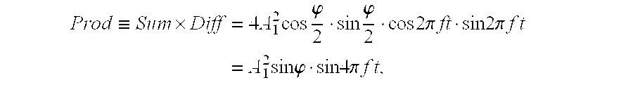


| TABLE A |
| Integration of a sine function |
| % error | Av. | Max. | |
| (based on 1000 simulations) | Errors (%) | S.D. Error (%) | Error (%) |
| Simpson Only | −3.73e−3 | 1.33e−3 | 6.17e−3 |
| Simpson + linear correction | 3.16e−8 | 4.89e−8 | 1.56e−7 |
| Simpson + quadratic correction | 2.00e−4 | 2.19e−2 | 5.18e−1 |
| TABLE B |
| Integration of a sine-squared function |
| % error | Av. | Max. | |
| (based on 1000 simulations | Errors (%) | S.D. Error (%) | Error (%) |
| Simpson Only | −2.21e−6 | 1.10e−6 | 4.39e−3 |
| Simpson + linear correction | 2.21e−6 | 6.93e−7 | 2.52e−6 |
| Simpson + quadratic correction | 2.15e−11 | 6.83e−11 | 1.88e−10 |


| TABLE C | ||
| Parameter | Value | Comment |
| ω | 160π | This corresponds to frequency = 80 Hz, a typical |
| value. | ||
| A1 | 0.1 | This more typically is 0.3, but it could be smaller with |
| aeration. | ||
| A2 | 0.01 | This more typically is 0.005, but it could be larger |
| with aeration. | ||
| A3 and A4 | 0.0 | The digital Coriolis simulation mode only offers two |
| harmonics, so these higher harmonics are ignored. | ||
| However, they are small (<0.002). | ||
| Z0 | 0.001 | Experience suggests that this is a large value for zero |
| offset. | ||
| εG | 0.001 | Experience suggests this is a large value for gain |
| mismatch. | ||
| TABLE D | |||
| Integral | ‘Exact’ Value | Estimate | Digital Coriolis Simulation |
| IIPs | 0.101353 | 0.101358 | 0.101340 |
| IINs | 0.098735 | 0.098740 | 0.098751 |
| IIPc | 0.007487 | 0.007488 | 0.007500 |
| IINc | −0.009496 | −0.009498 | −0.009531 |
| I2Ps | 0.009149 | 0.009151 | 0.009118 |
| I2Ns | 0.010857 | 0.010859 | 0.010885 |


| TABLE 1 | ||||
| Expected | Confidence | |||
| Persistence | in RMV | MV Status | ||
| not applicable | nominal | CLEAR | ||
| not applicable | reduced | BLURRED | ||
| short | zero | DAZZLED | ||
| long | zero | BLIND | ||
Claims (56)
Priority Applications (5)
| Application Number | Priority Date | Filing Date | Title |
|---|---|---|---|
| US09/931,002 US6507791B2 (en) | 1997-11-26 | 2001-08-17 | Digital flowmeter |
| US11/930,936 US8000906B2 (en) | 1997-11-26 | 2007-10-31 | Digital flowmeter |
| US12/852,008 US8467986B2 (en) | 1997-11-26 | 2010-08-06 | Drive techniques for a digital flowmeter |
| US13/198,313 US8447534B2 (en) | 1997-11-26 | 2011-08-04 | Digital flowmeter |
| US13/853,793 US9046400B2 (en) | 1997-11-26 | 2013-03-29 | Digital flowmeter |
Applications Claiming Priority (3)
| Application Number | Priority Date | Filing Date | Title |
|---|---|---|---|
| US6655497P | 1997-11-26 | 1997-11-26 | |
| US09/111,739 US6311136B1 (en) | 1997-11-26 | 1998-07-08 | Digital flowmeter |
| US09/931,002 US6507791B2 (en) | 1997-11-26 | 2001-08-17 | Digital flowmeter |
Related Parent Applications (1)
| Application Number | Title | Priority Date | Filing Date |
|---|---|---|---|
| US09/111,739 Continuation US6311136B1 (en) | 1997-11-26 | 1998-07-08 | Digital flowmeter |
Related Child Applications (1)
| Application Number | Title | Priority Date | Filing Date |
|---|---|---|---|
| US09/931,057 Continuation US6754594B2 (en) | 1997-11-26 | 2001-08-17 | Digital flowmeter |
Publications (2)
| Publication Number | Publication Date |
|---|---|
| US20020038186A1 US20020038186A1 (en) | 2002-03-28 |
| US6507791B2 true US6507791B2 (en) | 2003-01-14 |
Family
ID=26746870
Family Applications (7)
| Application Number | Title | Priority Date | Filing Date |
|---|---|---|---|
| US09/111,739 Expired - Lifetime US6311136B1 (en) | 1997-11-26 | 1998-07-08 | Digital flowmeter |
| US09/931,002 Expired - Lifetime US6507791B2 (en) | 1997-11-26 | 2001-08-17 | Digital flowmeter |
| US09/931,057 Expired - Lifetime US6754594B2 (en) | 1997-11-26 | 2001-08-17 | Digital flowmeter |
| US10/637,620 Expired - Lifetime US6917887B2 (en) | 1997-11-26 | 2003-08-11 | Digital flowmeter |
| US11/130,233 Expired - Lifetime US7136761B2 (en) | 1997-11-26 | 2005-05-17 | Digital flowmeter |
| US11/555,033 Expired - Fee Related US7571062B2 (en) | 1997-11-26 | 2006-10-31 | Digital flowmeter |
| US11/930,936 Expired - Fee Related US8000906B2 (en) | 1997-11-26 | 2007-10-31 | Digital flowmeter |
Family Applications Before (1)
| Application Number | Title | Priority Date | Filing Date |
|---|---|---|---|
| US09/111,739 Expired - Lifetime US6311136B1 (en) | 1997-11-26 | 1998-07-08 | Digital flowmeter |
Family Applications After (5)
| Application Number | Title | Priority Date | Filing Date |
|---|---|---|---|
| US09/931,057 Expired - Lifetime US6754594B2 (en) | 1997-11-26 | 2001-08-17 | Digital flowmeter |
| US10/637,620 Expired - Lifetime US6917887B2 (en) | 1997-11-26 | 2003-08-11 | Digital flowmeter |
| US11/130,233 Expired - Lifetime US7136761B2 (en) | 1997-11-26 | 2005-05-17 | Digital flowmeter |
| US11/555,033 Expired - Fee Related US7571062B2 (en) | 1997-11-26 | 2006-10-31 | Digital flowmeter |
| US11/930,936 Expired - Fee Related US8000906B2 (en) | 1997-11-26 | 2007-10-31 | Digital flowmeter |
Country Status (4)
| Country | Link |
|---|---|
| US (7) | US6311136B1 (en) |
| EP (1) | EP0919793B1 (en) |
| JP (2) | JP2000018995A (en) |
| DE (3) | DE69840766D1 (en) |
Cited By (23)
| Publication number | Priority date | Publication date | Assignee | Title |
|---|---|---|---|---|
| US20020129661A1 (en) * | 2001-01-16 | 2002-09-19 | Clarke David W. | Vortex flowmeter |
| US20030212509A1 (en) * | 2002-03-29 | 2003-11-13 | Henry Manus P. | Startup and operational techniques for a digital flowmeter |
| US20040031328A1 (en) * | 1997-11-26 | 2004-02-19 | The Foxboro Company | Digital flowmeter |
| US20040206189A1 (en) * | 2000-03-23 | 2004-10-21 | Invensys Systems, Inc. | Correcting for two-phase flow in a digital flowmeter |
| US20040221660A1 (en) * | 2003-05-05 | 2004-11-11 | Dutton Robert E. | Two-phase steam measurement system |
| WO2005003690A2 (en) * | 2003-06-26 | 2005-01-13 | Invensys Systems, Inc. | Viscosity-corrected flowmeter |
| US20050011282A1 (en) * | 2003-06-06 | 2005-01-20 | Voege James A. | Lighted fluid flow indication apparatus |
| US20050034537A1 (en) * | 2003-08-13 | 2005-02-17 | Henry Manus P. | Correcting frequency in flowtube measurements |
| US20050081643A1 (en) * | 2003-02-10 | 2005-04-21 | Mattar Wade M. | Multiphase coriolis flowmeter |
| US20050109123A1 (en) * | 2003-10-30 | 2005-05-26 | Robert Cheesewright | Dynamic response characteristics of flow meters |
| US20050126305A1 (en) * | 2003-12-12 | 2005-06-16 | Rosemount Inc. | Tunable empty pipe function |
| US20050193832A1 (en) * | 2003-02-10 | 2005-09-08 | Tombs Michael S. | Multi-phase Coriolis flowmeter |
| US20050274173A1 (en) * | 2004-05-27 | 2005-12-15 | Asml Holding N.V. | Gas gauge proximity sensor with a modulated gas flow |
| US20050284237A1 (en) * | 1997-11-26 | 2005-12-29 | Invensys Systems, Inc., A Massachusetts Corporation | Correcting for two-phase flow in a digital flowmeter |
| US20060179956A1 (en) * | 2005-02-16 | 2006-08-17 | Kolahi Kourosh | Method for operating a mass flowmeter |
| US20070006666A1 (en) * | 2005-07-11 | 2007-01-11 | Invensys Systems, Inc. | Coriolis mode processing techniques |
| US7404336B2 (en) | 2000-03-23 | 2008-07-29 | Invensys Systems, Inc. | Correcting for two-phase flow in a digital flowmeter |
| US20080252283A1 (en) * | 2005-10-18 | 2008-10-16 | Mcanally Craig B | Meter Electronics and Methods for Determining a Phase Difference Between a First Sensor Signal and a Second Sensor Signal of a Flow Meter |
| US20090019947A1 (en) * | 1999-11-22 | 2009-01-22 | Invensys Systems, Inc. | Correcting for Two-Phase Flow in a Digital Flowmeter |
| US20090090504A1 (en) * | 2007-10-05 | 2009-04-09 | Halliburton Energy Services, Inc. - Duncan | Determining Fluid Rheological Properties |
| US20110035166A1 (en) * | 1997-11-26 | 2011-02-10 | Invensys Systems, Inc. | Drive techniques for a digital flowmeter |
| US8126661B2 (en) | 2006-08-28 | 2012-02-28 | Henry Manus P | Wet gas measurement |
| US9046400B2 (en) | 1997-11-26 | 2015-06-02 | Invensys Systems, Inc. | Digital flowmeter |
Families Citing this family (200)
| Publication number | Priority date | Publication date | Assignee | Title |
|---|---|---|---|---|
| DE102013101369B4 (en) | 2013-02-12 | 2021-02-18 | Endress + Hauser Flowtec Ag | Coriolis mass flow meter |
| US6017143A (en) | 1996-03-28 | 2000-01-25 | Rosemount Inc. | Device in a process system for detecting events |
| US8290721B2 (en) | 1996-03-28 | 2012-10-16 | Rosemount Inc. | Flow measurement diagnostics |
| US7254518B2 (en) * | 1996-03-28 | 2007-08-07 | Rosemount Inc. | Pressure transmitter with diagnostics |
| US7949495B2 (en) | 1996-03-28 | 2011-05-24 | Rosemount, Inc. | Process variable transmitter with diagnostics |
| US6539267B1 (en) | 1996-03-28 | 2003-03-25 | Rosemount Inc. | Device in a process system for determining statistical parameter |
| US6754601B1 (en) | 1996-11-07 | 2004-06-22 | Rosemount Inc. | Diagnostics for resistive elements of process devices |
| US6601005B1 (en) * | 1996-11-07 | 2003-07-29 | Rosemount Inc. | Process device diagnostics using process variable sensor signal |
| US6519546B1 (en) | 1996-11-07 | 2003-02-11 | Rosemount Inc. | Auto correcting temperature transmitter with resistance based sensor |
| US6594620B1 (en) * | 1998-08-17 | 2003-07-15 | Aspen Technology, Inc. | Sensor validation apparatus and method |
| US6611775B1 (en) | 1998-12-10 | 2003-08-26 | Rosemount Inc. | Electrode leakage diagnostics in a magnetic flow meter |
| US6615149B1 (en) | 1998-12-10 | 2003-09-02 | Rosemount Inc. | Spectral diagnostics in a magnetic flow meter |
| US7010459B2 (en) * | 1999-06-25 | 2006-03-07 | Rosemount Inc. | Process device diagnostics using process variable sensor signal |
| US6505517B1 (en) | 1999-07-23 | 2003-01-14 | Rosemount Inc. | High accuracy signal processing for magnetic flowmeter |
| US6701274B1 (en) | 1999-08-27 | 2004-03-02 | Rosemount Inc. | Prediction of error magnitude in a pressure transmitter |
| US6543297B1 (en) | 1999-09-13 | 2003-04-08 | Rosemount Inc. | Process flow plate with temperature measurement feature |
| US6487507B1 (en) * | 1999-10-15 | 2002-11-26 | Micro Motion, Inc. | Remote signal conditioner for a Coriolis flowmeter |
| US6618684B1 (en) * | 2000-01-26 | 2003-09-09 | Elster Electricity, Llc | System and method for digitally compensating frequency and temperature induced errors in amplitude and phase shift in current sensing of electronic energy meters |
| DE10045537A1 (en) * | 2000-09-13 | 2002-03-21 | Flowtec Ag | Measuring and operating circuit for Coriolis mass flowmeter uses digital processor for calculation of mass flow rate using one oscillation sensor signal and difference between oscillation sensor signals |
| US6629059B2 (en) | 2001-05-14 | 2003-09-30 | Fisher-Rosemount Systems, Inc. | Hand held diagnostic and communication device with automatic bus detection |
| JP4202247B2 (en) * | 2001-06-19 | 2008-12-24 | エンドレス ウント ハウザー フローテック アクチエンゲゼルシャフト | Equipment for measuring viscosity |
| US6832179B2 (en) * | 2001-06-26 | 2004-12-14 | Invensys Systems, Inc. | Evaluating a vortex flow-meter signal |
| US6772036B2 (en) | 2001-08-30 | 2004-08-03 | Fisher-Rosemount Systems, Inc. | Control system using process model |
| US6606917B2 (en) * | 2001-11-26 | 2003-08-19 | Emerson Electric Co. | High purity coriolis mass flow controller |
| US20030098069A1 (en) * | 2001-11-26 | 2003-05-29 | Sund Wesley E. | High purity fluid delivery system |
| JP3753057B2 (en) * | 2001-12-04 | 2006-03-08 | 株式会社日立製作所 | Gas flow measuring device |
| JP3669580B2 (en) * | 2002-05-24 | 2005-07-06 | 学校法人慶應義塾 | Ultrasonic flow velocity distribution and flow meter |
| DE10223358A1 (en) * | 2002-05-25 | 2003-12-04 | Bosch Gmbh Robert | Method and arrangement for detecting the movement of an element |
| GB2391313B (en) * | 2002-07-26 | 2006-01-18 | Abb Ltd | Deriving measurements from periodic data |
| US7040179B2 (en) | 2002-12-06 | 2006-05-09 | Endress+ Hauser Flowtec Ag | Process meter |
| US6993396B1 (en) * | 2003-03-20 | 2006-01-31 | John Peter Gerry | System for determining the health of process control feedback loops according to performance assessment criteria |
| US6997032B2 (en) * | 2003-04-08 | 2006-02-14 | Invensys Systems, Inc. | Flowmeter zeroing techniques |
| DE10322763A1 (en) * | 2003-05-19 | 2004-12-09 | Helios + Zaschel Gmbh | Method and device for measuring a mass flow |
| DE10331126B4 (en) | 2003-07-09 | 2005-09-01 | Krohne Ag | Coriolis mass flowmeter and method of operating a Coriolis mass flowmeter |
| MXPA06003429A (en) * | 2003-09-30 | 2006-06-27 | Micro Motion Inc | Two-wire bus instrument. |
| US7124037B2 (en) * | 2003-10-31 | 2006-10-17 | Mpi Incorporated | Devices, systems, and methods for monitoring the operation of an injection molding machine |
| US7040181B2 (en) | 2004-03-19 | 2006-05-09 | Endress + Hauser Flowtec Ag | Coriolis mass measuring device |
| US20050274200A1 (en) * | 2004-05-25 | 2005-12-15 | Henry Manus P | Flowmeter batching techniques |
| US7302356B2 (en) * | 2004-09-15 | 2007-11-27 | Endress + Hauser Flowtec Ag | Coriolis flowmeter |
| DE102004060115A1 (en) * | 2004-12-13 | 2006-06-14 | Endress + Hauser Flowtec Ag | Transducer of the vibration type |
| US7350421B2 (en) * | 2004-12-13 | 2008-04-01 | Endress + Hauser Flowtec Ag | Vibratory measurement transducer |
| CN100554892C (en) * | 2004-12-29 | 2009-10-28 | 微动公司 | The fast frequency and the phase estimation that are used for flowmeter |
| US7064692B1 (en) * | 2005-03-18 | 2006-06-20 | Honeywell International Inc. | Solid-state synchro/resolver converter |
| IN266753B (en) * | 2005-03-29 | 2015-05-29 | Micro Motion Inc | |
| US8112565B2 (en) | 2005-06-08 | 2012-02-07 | Fisher-Rosemount Systems, Inc. | Multi-protocol field device interface with automatic bus detection |
| US7337084B2 (en) * | 2005-06-21 | 2008-02-26 | Invensys Systems, Inc. | Switch-activated zero checking feature for a Coriolis flowmeter |
| EP1925916A3 (en) | 2005-07-11 | 2011-08-03 | Invensys Systems, Inc. | Coriolis mode processing techniques |
| DE102005046319A1 (en) | 2005-09-27 | 2007-03-29 | Endress + Hauser Flowtec Ag | Two or multi-phase medium e.g. fluid`s, physical flow parameter e.g. flow rate, measuring method, involves producing measurement values representing parameter by considering pressure difference of medium and by usage of transfer function |
| US20070068225A1 (en) | 2005-09-29 | 2007-03-29 | Brown Gregory C | Leak detector for process valve |
| US7505947B2 (en) * | 2005-10-20 | 2009-03-17 | International Business Machines Corporation | Computer controlled method using genetic algorithms to provide non-deterministic solutions to problems involving physical restraints |
| US7360452B2 (en) * | 2005-12-27 | 2008-04-22 | Endress + Hauser Flowtec Ag | In-line measuring devices and method for compensation measurement errors in in-line measuring devices |
| CA2634959C (en) | 2005-12-27 | 2013-02-05 | Wolfgang Drahm | In-line measuring devices and method for compensating measurement errors in in-line measuring devices |
| US7360453B2 (en) * | 2005-12-27 | 2008-04-22 | Endress + Hauser Flowtec Ag | In-line measuring devices and method for compensation measurement errors in in-line measuring devices |
| US7532992B2 (en) * | 2006-01-20 | 2009-05-12 | Teledyne Isco, Inc. | Measuring apparatuses and methods of using them |
| EP1989517B1 (en) * | 2006-02-13 | 2015-09-02 | Invensys Systems, Inc. | Compensating for frequency change in flowmeters |
| WO2007130017A1 (en) * | 2006-04-28 | 2007-11-15 | Micro Motion, Inc. | Bus loop power interface and method |
| DE102006031198B4 (en) * | 2006-07-04 | 2012-01-26 | Krohne Ag | Method of operating a Coriolis mass flowmeter |
| JP2008027263A (en) * | 2006-07-24 | 2008-02-07 | Oval Corp | Processing method in arithmetic system, flow rate converter, and coriolis flowmeter |
| US7953501B2 (en) | 2006-09-25 | 2011-05-31 | Fisher-Rosemount Systems, Inc. | Industrial process control loop monitor |
| WO2008042290A2 (en) | 2006-09-29 | 2008-04-10 | Rosemount Inc. | Magnetic flowmeter with verification |
| DE102006058732A1 (en) | 2006-12-13 | 2008-06-26 | Abb Ag | Vibration type measurement device i.e. Coriolis measurement device, operating process, involves using phase shift as input for controller so that excitation frequency is automatically adjusted as function of phase shift |
| DE102006062600B4 (en) | 2006-12-29 | 2023-12-21 | Endress + Hauser Flowtec Ag | Method for commissioning and/or monitoring an in-line measuring device |
| AT9241U3 (en) * | 2007-02-05 | 2007-12-15 | Avl List Gmbh | METHOD AND DEVICE FOR CONTINUOUS MEASUREMENT OF DYNAMIC FLUID CONSUMPTION |
| WO2008109841A1 (en) * | 2007-03-07 | 2008-09-12 | Invensys Systems, Inc. | Coriolis frequency tracking |
| DE102007021099A1 (en) | 2007-05-03 | 2008-11-13 | Endress + Hauser (Deutschland) Ag + Co. Kg | Method for commissioning and / or reconfiguring a programmable field meter |
| WO2008147408A1 (en) * | 2007-05-25 | 2008-12-04 | Micro Motion, Inc. | Vibratory flow meter and method for correcting for entrained gas in a flow material |
| US8898036B2 (en) | 2007-08-06 | 2014-11-25 | Rosemount Inc. | Process variable transmitter with acceleration sensor |
| DE102007058608A1 (en) | 2007-12-04 | 2009-06-10 | Endress + Hauser Flowtec Ag | Electric device |
| US7895006B2 (en) * | 2007-12-21 | 2011-02-22 | Agilent Technologies, Inc. | System and method for determining signal-to-noise ratio (SNR), signal-to-noise and distortion ratio (SINAD) and total harmonic distortion (THD) |
| DE102008011381A1 (en) * | 2008-02-27 | 2009-09-03 | Endress + Hauser Flowtec Ag | Method for producing sinusoidal electric voltage waveform, involves producing discrete electrical signals, where discrete electrical signal assumes one of two voltage levels |
| DE102008016235A1 (en) | 2008-03-27 | 2009-10-01 | Endress + Hauser Flowtec Ag | A method of operating a meter disposed on a rotary carousel filling machine |
| KR101347781B1 (en) * | 2008-05-01 | 2014-02-13 | 마이크로 모우션, 인코포레이티드 | Very high frequency vibratory flow meter, method of operating the same and method of forming the same |
| DE102008022373A1 (en) | 2008-05-06 | 2009-11-12 | Endress + Hauser Flowtec Ag | Measuring device and method for monitoring a measuring device |
| US9354097B2 (en) * | 2008-07-01 | 2016-05-31 | Micro Motion, Inc. | System, method, and computer program product for generating a drive signal in a vibrating measuring device |
| DE102008035877A1 (en) | 2008-08-01 | 2010-02-04 | Endress + Hauser Flowtec Ag | Vibration-type transducers |
| DE102008050115A1 (en) | 2008-10-06 | 2010-04-08 | Endress + Hauser Flowtec Ag | In-line measuring device |
| DE102008050113A1 (en) | 2008-10-06 | 2010-04-08 | Endress + Hauser Flowtec Ag | In-line measuring device |
| DE102008050116A1 (en) | 2008-10-06 | 2010-04-08 | Endress + Hauser Flowtec Ag | In-line measuring device |
| DE102008044186A1 (en) | 2008-11-28 | 2010-06-02 | Endress + Hauser Flowtec Ag | Magnetic device and transducer of the vibration type with such a magnetic device |
| JP4436884B1 (en) * | 2009-02-06 | 2010-03-24 | 株式会社オーバル | Signal processing method, signal processing apparatus, and Coriolis flow meter |
| JP4436883B1 (en) * | 2009-02-06 | 2010-03-24 | 株式会社オーバル | Signal processing method, signal processing apparatus, and Coriolis flow meter |
| JP4436882B1 (en) * | 2009-02-06 | 2010-03-24 | 株式会社オーバル | Signal processing method, signal processing apparatus, and Coriolis flow meter |
| EP2406591A1 (en) | 2009-03-11 | 2012-01-18 | Endress+Hauser Flowtec AG | Vibration sensor and in-line measuring device comprising said sensor |
| DE102009001472A1 (en) | 2009-03-11 | 2010-09-16 | Endress + Hauser Flowtec Ag | Vibration-type transducers and in-line meter with such a transducer |
| DE102009027580A1 (en) | 2009-07-09 | 2011-01-13 | Endress + Hauser Flowtec Ag | Measuring system for use as compact Coriolis mass flow rate/vicosity measuring device to measure e.g. density of slurry flowing into process line, has measuring tubes executing diametrically opposed torsional vibrations in fundamental mode |
| DE102009012474A1 (en) | 2009-03-12 | 2010-09-16 | Endress + Hauser Flowtec Ag | Measuring system with a vibration-type transducer |
| US7921734B2 (en) | 2009-05-12 | 2011-04-12 | Rosemount Inc. | System to detect poor process ground connections |
| WO2011008307A1 (en) * | 2009-07-13 | 2011-01-20 | Micro Motion, Inc. | Meter electronics and fluid quantification method for a fluid being transferred |
| CN101608940B (en) * | 2009-07-23 | 2011-12-21 | 合肥工业大学 | Coriolis mass flowmeter plus-minus phase-step alternative excitation vibration-starting method and system thereof |
| DE102009028006A1 (en) | 2009-07-24 | 2011-01-27 | Endress + Hauser Flowtec Ag | Vibration-type transducers and measuring instrument with such a transducer |
| DE102009028007A1 (en) | 2009-07-24 | 2011-01-27 | Endress + Hauser Flowtec Ag | Measuring transducer of the vibration type and measuring device with such a transducer |
| CA2770135C (en) * | 2009-08-12 | 2016-06-07 | Micro Motion, Inc. | Method and apparatus for determining a zero offset in a vibrating flow meter |
| CA2769485C (en) * | 2009-08-12 | 2015-06-23 | Micro Motion, Inc. | Method and apparatus for determining and compensating for a change in a differential zero offset of a vibrating flow meter |
| DE102009046839A1 (en) | 2009-11-18 | 2011-05-19 | Endress + Hauser Flowtec Ag | Measuring system with a two parallel flowed measuring tubes having pipe assembly and method for monitoring thereof |
| DE102010039627A1 (en) | 2010-08-20 | 2012-02-23 | Endress + Hauser Flowtec Ag | Vibration-type measuring transducer for e.g. flow/density/viscosity measuring device, used for registering mass flow rate of medium flowing in pipeline, has imaginary longitudinal-section plane extending between respective measuring tubes |
| WO2011085851A1 (en) | 2009-12-21 | 2011-07-21 | Endress+Hauser Flowtec Ag | Vibration type sensor |
| DE102009055069A1 (en) | 2009-12-21 | 2011-06-22 | Endress + Hauser Flowtec Ag | Vibration-type measuring sensor for detecting e.g. mass flow rate of gas and for producing Coriolis forces in process measurement- and automation system, has tube arrangement exhibiting sectional plane running between measuring tubes |
| DE102010000760B4 (en) | 2010-01-11 | 2021-12-23 | Endress + Hauser Flowtec Ag | A measuring system comprising a transducer of the vibration type for measuring a static pressure in a flowing medium |
| DE102010000761A1 (en) | 2010-01-11 | 2011-07-28 | Endress + Hauser Flowtec Ag | Measuring system i.e. measuring device and/or Coriolis or mass flow measuring device for medium e.g. gas and/or liquid, flowing in pipeline, has transmitter electronics generating measured value |
| CA2785933C (en) | 2009-12-31 | 2016-05-24 | Endress+Hauser Flowtec Ag | Measuring system having a measuring transducer of vibration-type |
| EP2519806B1 (en) | 2009-12-31 | 2018-02-07 | Endress+Hauser Flowtec AG | Measuring system with vibration type transducer |
| DE102010000759A1 (en) | 2010-01-11 | 2011-07-14 | Endress + Hauser Flowtec Ag | Measuring system i.e. Coriolis mass flow measuring device, for measuring pressure difference of medium flowing in pipeline of industrial plant, has electronics housing generating measured value representing reynolds number for medium |
| CN102753946B (en) | 2009-12-31 | 2016-08-17 | 恩德斯+豪斯流量技术股份有限公司 | There is the measurement system of vibration-type measuring transducer |
| JP4694645B1 (en) * | 2010-02-19 | 2011-06-08 | 株式会社オーバル | Signal processing method, signal processing apparatus, and vibration type density meter |
| WO2011131399A1 (en) | 2010-04-19 | 2011-10-27 | Endress+Hauser Flowtec Ag | Driver circuit for a measuring transducer and measuring system designed having same |
| DE202010006553U1 (en) | 2010-05-06 | 2011-10-05 | Endress + Hauser Flowtec Ag | Electronic measuring device with an optocoupler |
| DE102010030924A1 (en) | 2010-06-21 | 2011-12-22 | Endress + Hauser Flowtec Ag | Electronics housing for an electronic device or device formed therewith |
| DE102010039543A1 (en) | 2010-08-19 | 2012-02-23 | Endress + Hauser Flowtec Ag | Measuring system with a vibration-type transducer |
| RU2551481C2 (en) | 2010-09-02 | 2015-05-27 | Эндресс+Хаузер Флоутек Аг | Measuring system for measurement of density and/or norm of mass flow rate and/or viscosity of fluid environment proceeding in pipeline and use of measuring system |
| CA2810448C (en) | 2010-09-16 | 2016-11-29 | Endress+Hauser Flowtec Ag | Measuring system having a measuring transducer of vibration type |
| DE102010044179A1 (en) | 2010-11-11 | 2012-05-16 | Endress + Hauser Flowtec Ag | Measuring system with a transducer of vibration type |
| CA2758779C (en) | 2010-12-01 | 2016-01-05 | Invensys Systems, Inc. | Determining concentrations of components of a mixture |
| WO2012089431A1 (en) | 2010-12-30 | 2012-07-05 | Endress+Hauser Flowtec Ag | Measuring sensor of the vibration type and measuring system formed thereby |
| US8593273B2 (en) | 2011-02-07 | 2013-11-26 | Infineon Technologies Ag | Systems and methods for localization of tire pressure monitoring system wheel modules |
| CN102128656B (en) * | 2011-02-25 | 2013-09-04 | 合肥工业大学 | Slightly bent Koch mass flow meter digital signal processing method and system |
| US9207670B2 (en) | 2011-03-21 | 2015-12-08 | Rosemount Inc. | Degrading sensor detection implemented within a transmitter |
| DE102011006971A1 (en) | 2011-04-07 | 2012-10-11 | Endress + Hauser Flowtec Ag | Vibration-type transducers and method of making same |
| DE102011006997A1 (en) | 2011-04-07 | 2012-10-11 | Endress + Hauser Flowtec Ag | Frequency adjustment method for a pipe arrangement |
| DE102011006919A1 (en) | 2011-04-07 | 2012-10-11 | Endress + Hauser Flowtec Ag | Method for trimming a pipe |
| JP5836628B2 (en) * | 2011-04-19 | 2015-12-24 | キヤノン株式会社 | Control system evaluation apparatus, evaluation method, and program |
| US8863589B2 (en) | 2011-05-02 | 2014-10-21 | Endress + Hauser Flowtec Ag | Measuring transducer of vibration type and measuring system |
| GB201108854D0 (en) * | 2011-05-26 | 2011-07-06 | Spp Process Technology Systems Uk Ltd | Mass flow controller monitoring |
| DE102011076838A1 (en) | 2011-05-31 | 2012-12-06 | Endress + Hauser Flowtec Ag | Meter electronics for a meter device and meter device formed thereby |
| EP2565594A1 (en) | 2011-07-11 | 2013-03-06 | Invensys Systems, Inc. | Coriolis flowmeter with zero checking feature |
| US20130080084A1 (en) * | 2011-09-28 | 2013-03-28 | John P. Miller | Pressure transmitter with diagnostics |
| US8565967B2 (en) * | 2011-12-21 | 2013-10-22 | Infineon Technologies Ag | Acceleration detection and angular position determination systems and methods in tire pressure monitoring systems |
| DE102011089808A1 (en) | 2011-12-23 | 2013-06-27 | Endress + Hauser Flowtec Ag | Method or measuring system for determining a density of a fluid |
| DE102012102947B4 (en) | 2012-04-03 | 2023-12-21 | Endress + Hauser Flowtec Ag | Vibration type transducer |
| RU2579818C1 (en) | 2012-04-03 | 2016-04-10 | Эндресс + Хаузер Флоутек Аг | Vibration-type measuring transducer, measuring system for medium flowing through pipeline and method for construction of frequency of system of pipes |
| EP2841879B1 (en) * | 2012-04-23 | 2021-06-02 | Rosemount Inc. | Process variable compensation in a process transmitter |
| WO2013189589A1 (en) * | 2012-06-18 | 2013-12-27 | Krohne Messtechnik Gmbh | Method for operating a resonant measurement system |
| US9052240B2 (en) | 2012-06-29 | 2015-06-09 | Rosemount Inc. | Industrial process temperature transmitter with sensor stress diagnostics |
| US9602122B2 (en) | 2012-09-28 | 2017-03-21 | Rosemount Inc. | Process variable measurement noise diagnostic |
| US9372107B2 (en) | 2012-10-11 | 2016-06-21 | Endress + Hauser Flowtec Ag | Measuring system for ascertaining a volume flow and/or a volume flow rate of a medium flowing in a pipeline |
| DE102012109729A1 (en) | 2012-10-12 | 2014-05-15 | Endress + Hauser Flowtec Ag | Measuring system for determining volumetric flow during measuring interval of total flowed volume of flowing medium, particularly liquid or gas, has vibration element for guiding flowing portion of medium, where vibration element has lumen |
| US9995666B2 (en) * | 2012-10-22 | 2018-06-12 | Rheonics Gmbh | Resonant sensors for fluid properties measurement |
| WO2014067059A1 (en) * | 2012-10-30 | 2014-05-08 | 西安东风机电有限公司 | Digital drive method and system of coriolis flow meter |
| WO2014078853A1 (en) | 2012-11-19 | 2014-05-22 | Invensys Systems, Inc. | Net oil and gas well test system |
| DE102013102708A1 (en) | 2013-03-18 | 2014-09-18 | Endress + Hauser Flowtec Ag | Vibration-type transducers and measuring system formed thereby |
| DE102013102711A1 (en) | 2013-03-18 | 2014-09-18 | Endress + Hauser Flowtec Ag | Vibration-type transducers and measuring system formed thereby |
| DE102013106157A1 (en) | 2013-06-13 | 2014-12-18 | Endress + Hauser Flowtec Ag | Measuring system with a pressure device and method for monitoring and / or checking such a pressure device |
| DE102013106155A1 (en) | 2013-06-13 | 2014-12-18 | Endress + Hauser Flowtec Ag | Measuring system with a pressure device and method for monitoring and / or checking such a pressure device |
| US10900348B2 (en) * | 2013-11-14 | 2021-01-26 | Micro Motion, Inc. | Coriolis direct wellhead measurement devices and methods |
| JP2015105929A (en) * | 2013-12-02 | 2015-06-08 | 株式会社東芝 | Electromagnetic flow meter |
| DE102013113689B4 (en) | 2013-12-09 | 2018-02-01 | Endress + Hauser Flowtec Ag | Density measuring device |
| DE102013114731A1 (en) | 2013-12-20 | 2015-06-25 | Endress+Hauser Flowtec Ag | Kitchen sink |
| EP3084367B1 (en) | 2013-12-20 | 2020-10-14 | Endress+Hauser Flowtec AG | Coil |
| DE102013021915A1 (en) | 2013-12-27 | 2015-07-02 | Endress + Hauser Flowtec Ag | Transducer of the vibration type |
| DE102014103427A1 (en) | 2014-03-13 | 2015-09-17 | Endress + Hauser Flowtec Ag | Converter device and thus formed measuring system |
| DE102014103430A1 (en) | 2014-03-13 | 2015-09-17 | Endress + Hauser Flowtec Ag | Converter device and thus formed measuring system |
| RU2663092C1 (en) * | 2014-09-04 | 2018-08-01 | Майкро Моушн, Инк. | Differential flowmeter |
| DE102015103208A1 (en) | 2014-10-17 | 2016-04-21 | Endress + Hauser Flowtec Ag | Measuring system for measuring at least one measured variable of a fluid and method for operating such a measuring system |
| US9689736B2 (en) | 2014-10-31 | 2017-06-27 | Invensys Systems, Inc. | Method to provide a quality measure for meter verification results |
| DE102014119212A1 (en) * | 2014-12-19 | 2016-06-23 | Endress + Hauser Flowtec Ag | Measuring arrangement and method for measuring the density of flowable media |
| CN107110752B (en) | 2014-12-30 | 2020-04-28 | 恩德斯+豪斯流量技术股份有限公司 | Method for measuring fluid density |
| DE102014019396A1 (en) | 2014-12-30 | 2016-06-30 | Endress+Hauser Flowtec Ag | Method for measuring a density of a fluid |
| JP6036864B2 (en) * | 2015-02-05 | 2016-11-30 | 横河電機株式会社 | Resonance circuit of measuring device |
| US9863798B2 (en) | 2015-02-27 | 2018-01-09 | Schneider Electric Systems Usa, Inc. | Systems and methods for multiphase flow metering accounting for dissolved gas |
| US10408655B2 (en) * | 2015-03-13 | 2019-09-10 | Micro Motion, Inc. | Temperature compensation of a signal in a vibratory meter |
| US9664548B2 (en) | 2015-03-19 | 2017-05-30 | Invensys Systems, Inc. | Testing system for petroleum wells having a fluidic system including a gas leg, a liquid leg, and bypass conduits in communication with multiple multiphase flow metering systems with valves to control fluid flow through the fluidic system |
| JP6495537B2 (en) * | 2015-07-27 | 2019-04-03 | マイクロ モーション インコーポレイテッド | Off-resonance cycling of Coriolis flow meters |
| US10408647B2 (en) * | 2016-02-15 | 2019-09-10 | Olea Networks, Inc. | Analysis of pipe systems with sensor devices |
| US10024707B2 (en) * | 2016-02-17 | 2018-07-17 | Schneider Electric Systems Usa, Inc. | Electromagnetic flowmeter calibration verification |
| EP3420321B1 (en) * | 2016-02-26 | 2022-08-10 | Micro Motion, Inc. | Meter electronics for two or more meter assemblies |
| DE102016112600A1 (en) | 2016-07-08 | 2018-01-11 | Endress + Hauser Flowtec Ag | measuring system |
| DE102016112599A1 (en) | 2016-07-08 | 2018-01-11 | Endress + Hauser Flowtec Ag | measuring system |
| DE102016114860A1 (en) | 2016-08-10 | 2018-02-15 | Endress + Hauser Flowtec Ag | Driver circuit and thus formed converter electronics or thus formed measuring system |
| US11790034B2 (en) | 2016-11-11 | 2023-10-17 | Oxford University Innovation Limited | Method and system for tracking sinusoidal wave parameters from a received signal that includes noise |
| EP3563123A1 (en) | 2016-12-29 | 2019-11-06 | Endress+Hauser Flowtec AG | Vibronic measuring system for measuring a mass flow rate |
| CN110114641B (en) | 2016-12-29 | 2021-08-03 | 恩德斯+豪斯流量技术股份有限公司 | Electronic vibration measurement system for measuring mass flow rate |
| DE102017106211A1 (en) | 2016-12-29 | 2018-07-05 | Endress+Hauser Flowtec Ag | Vibronic measuring system for measuring a mass flow rate |
| CN106643955B (en) * | 2017-02-20 | 2023-04-07 | 重庆机床(集团)有限责任公司 | Flow monitoring controller |
| DE102017121157A1 (en) | 2017-08-09 | 2019-02-14 | Endress+Hauser Flowtec Ag | Coil and transducer with such a coil |
| DE102017118109A1 (en) | 2017-08-09 | 2019-02-14 | Endress + Hauser Flowtec Ag | sensor assembly |
| DE102018102831A1 (en) | 2017-10-05 | 2019-04-11 | Endress+Hauser Flowtec Ag | Transducer for a vibronic measuring system and thus formed vibronic measuring system |
| DE102017125273A1 (en) * | 2017-10-27 | 2019-05-02 | Endress + Hauser Flowtec Ag | Mass flowmeter according to the Coriolis principle with at least two measuring tube pairs and method for determining the mass flow |
| DE102017125271A1 (en) * | 2017-10-27 | 2019-05-02 | Endress + Hauser Flowtec Ag | Mass flowmeter according to the Coriolis principle with at least two measuring tube pairs |
| DE102017131199A1 (en) | 2017-12-22 | 2019-06-27 | Endress + Hauser Flowtec Ag | Coriolis mass flow meter |
| US11237550B2 (en) | 2018-03-28 | 2022-02-01 | Honeywell International Inc. | Ultrasonic flow meter prognostics with near real-time condition based uncertainty analysis |
| US11781673B2 (en) * | 2018-04-30 | 2023-10-10 | Keto A.I., Inc. | Water level control system |
| CN113242960A (en) | 2018-12-20 | 2021-08-10 | 恩德斯+豪斯流量技术股份有限公司 | Coriolis mass flowmeter |
| DE102018133117A1 (en) | 2018-12-20 | 2020-06-25 | Endress+Hauser Flowtec Ag | Coriolis mass flow meter |
| US20220099543A1 (en) | 2018-12-20 | 2022-03-31 | Endress+Hauser Flowtec Ag | Coriolis mass flow meter |
| WO2020126286A1 (en) | 2018-12-21 | 2020-06-25 | Endress+Hauser Flowtec Ag | Coriolis mass flowmeter with magnetic field detector |
| US20200209031A1 (en) * | 2018-12-26 | 2020-07-02 | Texas Instruments Incorporated | Dynamic temperature calibration of ultrasonic transducers |
| WO2020159950A1 (en) * | 2019-01-28 | 2020-08-06 | The Texas A&M University System | Method and device to measure multiphase flow |
| CN110346006A (en) * | 2019-08-13 | 2019-10-18 | 上海一诺仪表有限公司 | A kind of mass flowmenter transmitter and mass flowmenter |
| CN110470347B (en) * | 2019-09-12 | 2021-12-17 | 上海旗浪节能环保科技有限公司 | A pipeline real-time supervision device for ocean steamer air conditioning system |
| DE102019124709A1 (en) * | 2019-09-13 | 2021-03-18 | Endress+Hauser Flowtec Ag | Method for operating a measuring device with at least one oscillator and measuring device for carrying out the method |
| DE102019133610A1 (en) | 2019-12-09 | 2021-06-10 | Endress + Hauser Flowtec Ag | Vibronic measuring system for measuring a mass flow of a fluid to be measured |
| DE102019009024A1 (en) | 2019-12-30 | 2021-07-01 | Endress+Hauser Flowtec Ag | Vibronic measuring system |
| WO2021255034A1 (en) | 2020-06-18 | 2021-12-23 | Endress+Hauser Flowtec Ag | Vibronic measuring system |
| DE102020120054A1 (en) | 2020-07-29 | 2022-02-03 | Endress + Hauser Flowtec Ag | Method for determining a fluid temperature and measuring system for it |
| DE102020131649A1 (en) | 2020-09-03 | 2022-03-03 | Endress + Hauser Flowtec Ag | Vibronic measuring system |
| DE102020127382A1 (en) | 2020-10-16 | 2022-04-21 | Endress+Hauser Flowtec Ag | Procedure for checking a vibronic measuring system |
| DE102021113360A1 (en) | 2021-05-21 | 2022-11-24 | Endress + Hauser Flowtec Ag | Vibronic measuring system |
| DE102021123412A1 (en) * | 2021-09-09 | 2023-03-09 | Endress+Hauser Flowtec Ag | Vibronic sensor for mass flow and density measurement |
| DE102022112523A1 (en) | 2022-05-18 | 2023-11-23 | Endress+Hauser Flowtec Ag | Vibronic measuring system |
| DE102022116111A1 (en) | 2022-06-28 | 2023-12-28 | Endress+Hauser Flowtec Ag | Vibronic measuring system |
| DE102022119145A1 (en) | 2022-07-29 | 2024-02-01 | Endress+Hauser Flowtec Ag | Connection circuit for a field device and field device |
Citations (40)
| Publication number | Priority date | Publication date | Assignee | Title |
|---|---|---|---|---|
| US3956682A (en) * | 1974-03-28 | 1976-05-11 | Pennwalt Corporation | Two-wire position-to-D.C. current transducer |
| USRE29383E (en) | 1974-01-10 | 1977-09-06 | Process Systems, Inc. | Digital fluid flow rate measurement or control system |
| USRE31450E (en) | 1977-07-25 | 1983-11-29 | Micro Motion, Inc. | Method and structure for flow measurement |
| US4419898A (en) * | 1980-10-17 | 1983-12-13 | Sarasota Automation Limited | Method and apparatus for determining the mass flow of a fluid |
| US4422338A (en) | 1981-02-17 | 1983-12-27 | Micro Motion, Inc. | Method and apparatus for mass flow measurement |
| US4491025A (en) | 1982-11-03 | 1985-01-01 | Micro Motion, Inc. | Parallel path Coriolis mass flow rate meter |
| US4727746A (en) | 1985-12-31 | 1988-03-01 | Horiba, Ltd. | Method of modal mass analysis of exhaust gas from a motor vehicle |
| US4782711A (en) * | 1986-10-14 | 1988-11-08 | K-Flow Division Of Kane Steel Co., Inc. | Method and apparatus for measuring mass flow |
| US4817448A (en) | 1986-09-03 | 1989-04-04 | Micro Motion, Inc. | Auto zero circuit for flow meter |
| US4823614A (en) * | 1986-04-28 | 1989-04-25 | Dahlin Erik B | Coriolis-type mass flowmeter |
| US4852410A (en) | 1986-10-03 | 1989-08-01 | Schlumberger Industries, Inc. | Omega-shaped, coriolis-type mass flow rate meter |
| US4879111A (en) | 1986-04-17 | 1989-11-07 | Cetus Corporation | Treatment of infections with lymphokines |
| US4891991A (en) | 1986-10-28 | 1990-01-09 | The Foxboro Company | Coriolis-type mass flowmeter |
| US4911006A (en) | 1986-10-03 | 1990-03-27 | Micro Motion Incorporated | Custody transfer meter |
| US4911020A (en) | 1986-10-28 | 1990-03-27 | The Foxboro Company | Coriolis-type mass flowmeter circuitry |
| US4934195A (en) | 1986-06-10 | 1990-06-19 | The Foxboro Company | Coriolis mass flowmeter |
| US4934196A (en) * | 1989-06-02 | 1990-06-19 | Micro Motion, Inc. | Coriolis mass flow rate meter having a substantially increased noise immunity |
| US4996871A (en) | 1989-06-02 | 1991-03-05 | Micro Motion, Inc. | Coriolis densimeter having substantially increased noise immunity |
| US5027662A (en) | 1987-07-15 | 1991-07-02 | Micro Motion, Inc. | Accuracy mass flow meter with asymmetry and viscous damping compensation |
| US5050439A (en) | 1986-10-28 | 1991-09-24 | The Foxboro Company | Coriolis-type mass flowmeter circuitry |
| US5054326A (en) | 1990-03-05 | 1991-10-08 | The Foxboro Company | Density compensator for coriolis-type mass flowmeters |
| US5218869A (en) | 1992-01-14 | 1993-06-15 | Diasonics, Inc. | Depth dependent bandpass of ultrasound signals using heterodyne mixing |
| US5228327A (en) | 1991-07-11 | 1993-07-20 | Micro Motion, Inc. | Technique for determining a mechanical zero value for a coriolis meter |
| US5271281A (en) | 1986-10-28 | 1993-12-21 | The Foxboro Company | Coriolis-type mass flowmeter |
| US5343764A (en) | 1986-10-28 | 1994-09-06 | The Foxboro Company | Coriolis-type mass flowmeter |
| US5347874A (en) | 1993-01-25 | 1994-09-20 | Micro Motion, Incorporated | In-flow coriolis effect mass flowmeter |
| US5400653A (en) | 1991-12-23 | 1995-03-28 | Micro Motion, Inc. | Coriolis effect meter using optical fiber sensors |
| US5429002A (en) | 1994-05-11 | 1995-07-04 | Schlumberger Industries, Inc. | Coriolis-type fluid mass flow rate measurement device and method employing a least-squares algorithm |
| US5469748A (en) | 1994-07-20 | 1995-11-28 | Micro Motion, Inc. | Noise reduction filter system for a coriolis flowmeter |
| US5497666A (en) | 1994-07-20 | 1996-03-12 | Micro Motion, Inc. | Increased sensitivity coriolis effect flowmeter using nodal-proximate sensors |
| US5497665A (en) | 1991-02-05 | 1996-03-12 | Direct Measurement Corporation | Coriolis mass flow rate meter having adjustable pressure and density sensitivity |
| US5555190A (en) | 1995-07-12 | 1996-09-10 | Micro Motion, Inc. | Method and apparatus for adaptive line enhancement in Coriolis mass flow meter measurement |
| US5570300A (en) | 1992-04-22 | 1996-10-29 | The Foxboro Company | Self-validating sensors |
| US5578764A (en) | 1994-07-11 | 1996-11-26 | Yokogawa Electric Corporation | Coriolis type mass flowmeter utilizing phase shifters for phase shifting of the output signals |
| US5594180A (en) | 1994-08-12 | 1997-01-14 | Micro Motion, Inc. | Method and apparatus for fault detection and correction in Coriolis effect mass flowmeters |
| US5687100A (en) * | 1996-07-16 | 1997-11-11 | Micro Motion, Inc. | Vibrating tube densimeter |
| US5774378A (en) | 1993-04-21 | 1998-06-30 | The Foxboro Company | Self-validating sensors |
| US5804741A (en) | 1996-11-08 | 1998-09-08 | Schlumberger Industries, Inc. | Digital phase locked loop signal processing for coriolis mass flow meter |
| US5926096A (en) | 1996-03-11 | 1999-07-20 | The Foxboro Company | Method and apparatus for correcting for performance degrading factors in a coriolis-type mass flowmeter |
| US6092429A (en) | 1997-12-04 | 2000-07-25 | Micro Motion, Inc. | Driver for oscillating a vibrating conduit |
Family Cites Families (50)
| Publication number | Priority date | Publication date | Assignee | Title |
|---|---|---|---|---|
| US31450A (en) * | 1861-02-19 | Improvement in tools used in the manufacture of iron | ||
| US29383A (en) * | 1860-07-31 | Improvement in preserving food | ||
| US5732193A (en) * | 1909-01-26 | 1998-03-24 | Aberson; Michael | Method and apparatus for behavioristic-format coding of quantitative resource data/distributed automation protocol |
| US4027662A (en) * | 1973-07-11 | 1977-06-07 | Milstein Medical Research Foundation, Inc. | Automatic blood pressure recorder |
| GB1583545A (en) * | 1976-08-04 | 1981-01-28 | Martin Sanchez J | Control systems |
| US4187721A (en) * | 1977-07-25 | 1980-02-12 | S & F Associates | Method and structure for flow measurement |
| DE3464189D1 (en) | 1984-08-03 | 1987-07-16 | Itt Ind Gmbh Deutsche | Videorecorder with a magnetic tape storage medium |
| US4773257A (en) | 1985-06-24 | 1988-09-27 | Chevron Research Company | Method and apparatus for testing the outflow from hydrocarbon wells on site |
| US4688418A (en) | 1985-10-17 | 1987-08-25 | Texaco Inc. | Method and apparatus for determining mass flow rate and quality in a steam line |
| DE8712331U1 (en) | 1986-09-26 | 1988-01-28 | Flowtec Ag, Reinach, Basel, Ch | |
| IT1213434B (en) | 1986-12-23 | 1989-12-20 | Nuovo Pignone S P A Ind Meccan | PROCEDURE PERFECTED FOR THE MEASUREMENT OF WEIGHT CAPACITIES AND RELATED DEVICES. |
| US5052231A (en) | 1988-05-19 | 1991-10-01 | Rheometron Ag | Mass flow gauge for flowing media with devices for determination of the Coriolis force |
| US4852409A (en) * | 1988-06-09 | 1989-08-01 | Fischer & Porter Company | Signal recovery system for mass flowmeter |
| US4879911A (en) | 1988-07-08 | 1989-11-14 | Micro Motion, Incorporated | Coriolis mass flow rate meter having four pulse harmonic rejection |
| US4852395A (en) * | 1988-12-08 | 1989-08-01 | Atlantic Richfield Company | Three phase fluid flow measuring system |
| US5029482A (en) | 1989-02-03 | 1991-07-09 | Chevron Research Company | Gas/liquid flow measurement using coriolis-based flow meters |
| MX171455B (en) * | 1989-06-09 | 1993-10-27 | Micro Motion Inc | IMPROVED MASS FLOW METER FOR FLUID MATERIALS WHERE THE SPEED OF MASS FLOW IS DETERMINED BASED ON THE CORIOLIS EFFECT |
| US5259250A (en) | 1990-05-14 | 1993-11-09 | Atlantic Richfield Company | Multi-phase fluid flow mesurement |
| US5054313A (en) * | 1990-07-17 | 1991-10-08 | National Metal And Refining Company, Ltd. | Control circuitry for viscosity sensors |
| JP2525085B2 (en) * | 1991-02-19 | 1996-08-14 | 株式会社クラレ | Iron manufacturing method |
| JP3040816B2 (en) * | 1991-03-30 | 2000-05-15 | 和廣 岡田 | Operation test method in device for detecting physical quantity using change in distance between electrodes, and physical quantity detection device having function of performing this method |
| JPH0820295B2 (en) * | 1991-08-01 | 1996-03-04 | マイクロ モーション,インコーポレイティド | Coriolis effect mass flow meter |
| US5295084A (en) * | 1991-10-08 | 1994-03-15 | Micromotion, Inc. | Vibrating tube densimeter |
| US5309342A (en) * | 1993-03-02 | 1994-05-03 | Cooper Industries, Inc. | Recessed lighting fixture |
| WO1995010028A1 (en) | 1993-10-05 | 1995-04-13 | Atlantic Richfield Company | Multiphase flowmeter for measuring flow rates and densities |
| JP2651891B2 (en) * | 1993-11-05 | 1997-09-10 | 株式会社日本開発コンサルタント | Circular metal strip tension applying device |
| JPH07169833A (en) * | 1993-12-14 | 1995-07-04 | Nec Corp | Semiconductor device and manufacture thereof |
| EP0698783A1 (en) | 1994-08-16 | 1996-02-28 | Endress + Hauser Flowtec AG | Evaluation electronics of a coriolis mass flow sensor |
| EP1229309A3 (en) | 1994-09-13 | 2003-02-05 | Fuji Electric Co., Ltd. | Phase difference measuring apparatus and mass flowmeter thereof |
| US5654502A (en) | 1995-12-28 | 1997-08-05 | Micro Motion, Inc. | Automatic well test system and method of operating the same |
| US5676461A (en) * | 1996-03-18 | 1997-10-14 | M. A. Hanna Rubber Compounding A Division Of M. A. Hanna Company | Oil injection apparatus and method for polymer processing |
| US5877954A (en) * | 1996-05-03 | 1999-03-02 | Aspen Technology, Inc. | Hybrid linear-neural network process control |
| US5734112A (en) * | 1996-08-14 | 1998-03-31 | Micro Motion, Inc. | Method and apparatus for measuring pressure in a coriolis mass flowmeter |
| US6073495A (en) | 1997-03-21 | 2000-06-13 | Endress + Hauser Flowtec Ag | Measuring and operating circuit of a coriolis-type mass flow meter |
| US6185470B1 (en) | 1997-11-07 | 2001-02-06 | Mcdonnell Douglas Corporation | Neural network predictive control method and system |
| US6311136B1 (en) * | 1997-11-26 | 2001-10-30 | Invensys Systems, Inc. | Digital flowmeter |
| US5969495A (en) * | 1997-12-31 | 1999-10-19 | Daewood Heavy Industries Ltd. | Accelerator device for electromotive vehicles |
| US6102846A (en) | 1998-02-26 | 2000-08-15 | Eastman Kodak Company | System and method of managing a psychological state of an individual using images |
| WO1999065810A1 (en) * | 1998-06-12 | 1999-12-23 | Maschinenfabrik Rieter Ag | Yarn changing method |
| WO2000010059A1 (en) | 1998-08-17 | 2000-02-24 | Aspen Technology, Inc. | Sensor validation apparatus and method |
| US6327914B1 (en) * | 1998-09-30 | 2001-12-11 | Micro Motion, Inc. | Correction of coriolis flowmeter measurements due to multiphase flows |
| US5969264A (en) * | 1998-11-06 | 1999-10-19 | Technology Commercialization Corp. | Method and apparatus for total and individual flow measurement of a single-or multi-phase medium |
| US6301973B1 (en) * | 1999-04-30 | 2001-10-16 | The United States Of America As Represented By The Administrator Of The National Aeronautics And Space Administration | Non-intrusive pressure/multipurpose sensor and method |
| US6318186B1 (en) * | 1999-06-28 | 2001-11-20 | Micro Motion, Inc. | Type identification and parameter selection for drive control in a coriolis flowmeter |
| US6505131B1 (en) * | 1999-06-28 | 2003-01-07 | Micro Motion, Inc. | Multi-rate digital signal processor for signals from pick-offs on a vibrating conduit |
| US6318156B1 (en) * | 1999-10-28 | 2001-11-20 | Micro Motion, Inc. | Multiphase flow measurement system |
| US6551251B2 (en) * | 2000-02-14 | 2003-04-22 | The United States Of America As Represented By The Administrator Of The National Aeronautics And Space Administration | Passive fetal heart monitoring system |
| WO2001071291A1 (en) * | 2000-03-23 | 2001-09-27 | Invensys Systems, Inc. | Correcting for two-phase flow in a digital flowmeter |
| US6378354B1 (en) * | 2000-07-21 | 2002-04-30 | Micro Motion, Inc. | System for calibrating a drive signal in a coriolis flowmeter to cause the driver to vibrate a conduit in a desired mode of vibration |
| US6505135B2 (en) * | 2001-03-13 | 2003-01-07 | Micro Motion, Inc. | Initialization algorithm for drive control in a coriolis flowmeter |
-
1998
- 1998-07-08 US US09/111,739 patent/US6311136B1/en not_active Expired - Lifetime
- 1998-11-26 DE DE69840766T patent/DE69840766D1/en not_active Expired - Lifetime
- 1998-11-26 DE DE98309694T patent/DE98309694T1/en active Pending
- 1998-11-26 DE DE69841903T patent/DE69841903D1/en not_active Expired - Lifetime
- 1998-11-26 JP JP10378592A patent/JP2000018995A/en not_active Withdrawn
- 1998-11-26 EP EP98309694A patent/EP0919793B1/en not_active Expired - Lifetime
-
2001
- 2001-08-17 US US09/931,002 patent/US6507791B2/en not_active Expired - Lifetime
- 2001-08-17 US US09/931,057 patent/US6754594B2/en not_active Expired - Lifetime
-
2003
- 2003-08-11 US US10/637,620 patent/US6917887B2/en not_active Expired - Lifetime
-
2005
- 2005-05-17 US US11/130,233 patent/US7136761B2/en not_active Expired - Lifetime
-
2006
- 2006-10-31 US US11/555,033 patent/US7571062B2/en not_active Expired - Fee Related
-
2007
- 2007-07-04 JP JP2007176131A patent/JP2007248479A/en active Pending
- 2007-10-31 US US11/930,936 patent/US8000906B2/en not_active Expired - Fee Related
Patent Citations (43)
| Publication number | Priority date | Publication date | Assignee | Title |
|---|---|---|---|---|
| USRE29383E (en) | 1974-01-10 | 1977-09-06 | Process Systems, Inc. | Digital fluid flow rate measurement or control system |
| US3956682A (en) * | 1974-03-28 | 1976-05-11 | Pennwalt Corporation | Two-wire position-to-D.C. current transducer |
| USRE31450E (en) | 1977-07-25 | 1983-11-29 | Micro Motion, Inc. | Method and structure for flow measurement |
| US4419898A (en) * | 1980-10-17 | 1983-12-13 | Sarasota Automation Limited | Method and apparatus for determining the mass flow of a fluid |
| US4422338A (en) | 1981-02-17 | 1983-12-27 | Micro Motion, Inc. | Method and apparatus for mass flow measurement |
| US4422338B1 (en) | 1981-02-17 | 1987-07-14 | ||
| US4491025A (en) | 1982-11-03 | 1985-01-01 | Micro Motion, Inc. | Parallel path Coriolis mass flow rate meter |
| US4491025B1 (en) | 1982-11-03 | 1988-01-05 | ||
| US4727746A (en) | 1985-12-31 | 1988-03-01 | Horiba, Ltd. | Method of modal mass analysis of exhaust gas from a motor vehicle |
| US4879111A (en) | 1986-04-17 | 1989-11-07 | Cetus Corporation | Treatment of infections with lymphokines |
| US4823614A (en) * | 1986-04-28 | 1989-04-25 | Dahlin Erik B | Coriolis-type mass flowmeter |
| US4934195A (en) | 1986-06-10 | 1990-06-19 | The Foxboro Company | Coriolis mass flowmeter |
| US4817448A (en) | 1986-09-03 | 1989-04-04 | Micro Motion, Inc. | Auto zero circuit for flow meter |
| US4852410A (en) | 1986-10-03 | 1989-08-01 | Schlumberger Industries, Inc. | Omega-shaped, coriolis-type mass flow rate meter |
| US4911006A (en) | 1986-10-03 | 1990-03-27 | Micro Motion Incorporated | Custody transfer meter |
| US4782711A (en) * | 1986-10-14 | 1988-11-08 | K-Flow Division Of Kane Steel Co., Inc. | Method and apparatus for measuring mass flow |
| US4891991A (en) | 1986-10-28 | 1990-01-09 | The Foxboro Company | Coriolis-type mass flowmeter |
| US4911020A (en) | 1986-10-28 | 1990-03-27 | The Foxboro Company | Coriolis-type mass flowmeter circuitry |
| US5271281A (en) | 1986-10-28 | 1993-12-21 | The Foxboro Company | Coriolis-type mass flowmeter |
| EP0696726A2 (en) | 1986-10-28 | 1996-02-14 | The Foxboro Company | Coriolis-type mass flowmeter |
| US5343764A (en) | 1986-10-28 | 1994-09-06 | The Foxboro Company | Coriolis-type mass flowmeter |
| US5050439A (en) | 1986-10-28 | 1991-09-24 | The Foxboro Company | Coriolis-type mass flowmeter circuitry |
| US5027662A (en) | 1987-07-15 | 1991-07-02 | Micro Motion, Inc. | Accuracy mass flow meter with asymmetry and viscous damping compensation |
| US4934196A (en) * | 1989-06-02 | 1990-06-19 | Micro Motion, Inc. | Coriolis mass flow rate meter having a substantially increased noise immunity |
| US4996871A (en) | 1989-06-02 | 1991-03-05 | Micro Motion, Inc. | Coriolis densimeter having substantially increased noise immunity |
| US5054326A (en) | 1990-03-05 | 1991-10-08 | The Foxboro Company | Density compensator for coriolis-type mass flowmeters |
| US5497665A (en) | 1991-02-05 | 1996-03-12 | Direct Measurement Corporation | Coriolis mass flow rate meter having adjustable pressure and density sensitivity |
| US5228327A (en) | 1991-07-11 | 1993-07-20 | Micro Motion, Inc. | Technique for determining a mechanical zero value for a coriolis meter |
| US5400653A (en) | 1991-12-23 | 1995-03-28 | Micro Motion, Inc. | Coriolis effect meter using optical fiber sensors |
| US5218869A (en) | 1992-01-14 | 1993-06-15 | Diasonics, Inc. | Depth dependent bandpass of ultrasound signals using heterodyne mixing |
| US5570300A (en) | 1992-04-22 | 1996-10-29 | The Foxboro Company | Self-validating sensors |
| US5347874A (en) | 1993-01-25 | 1994-09-20 | Micro Motion, Incorporated | In-flow coriolis effect mass flowmeter |
| US5774378A (en) | 1993-04-21 | 1998-06-30 | The Foxboro Company | Self-validating sensors |
| US5429002A (en) | 1994-05-11 | 1995-07-04 | Schlumberger Industries, Inc. | Coriolis-type fluid mass flow rate measurement device and method employing a least-squares algorithm |
| US5578764A (en) | 1994-07-11 | 1996-11-26 | Yokogawa Electric Corporation | Coriolis type mass flowmeter utilizing phase shifters for phase shifting of the output signals |
| US5497666A (en) | 1994-07-20 | 1996-03-12 | Micro Motion, Inc. | Increased sensitivity coriolis effect flowmeter using nodal-proximate sensors |
| US5469748A (en) | 1994-07-20 | 1995-11-28 | Micro Motion, Inc. | Noise reduction filter system for a coriolis flowmeter |
| US5594180A (en) | 1994-08-12 | 1997-01-14 | Micro Motion, Inc. | Method and apparatus for fault detection and correction in Coriolis effect mass flowmeters |
| US5555190A (en) | 1995-07-12 | 1996-09-10 | Micro Motion, Inc. | Method and apparatus for adaptive line enhancement in Coriolis mass flow meter measurement |
| US5926096A (en) | 1996-03-11 | 1999-07-20 | The Foxboro Company | Method and apparatus for correcting for performance degrading factors in a coriolis-type mass flowmeter |
| US5687100A (en) * | 1996-07-16 | 1997-11-11 | Micro Motion, Inc. | Vibrating tube densimeter |
| US5804741A (en) | 1996-11-08 | 1998-09-08 | Schlumberger Industries, Inc. | Digital phase locked loop signal processing for coriolis mass flow meter |
| US6092429A (en) | 1997-12-04 | 2000-07-25 | Micro Motion, Inc. | Driver for oscillating a vibrating conduit |
Non-Patent Citations (6)
| Title |
|---|
| Henry, M. P. Signal Processing, Data Handling and Communications: The Case for Measurement Validation. Mar. 1992.* * |
| M. Henry et al., "The Implications of Digital Communications on Sensor Validation", Report No. QUEL 1912/92, University of Oxford, Department of Engineering Science, Apr. 1992. |
| M.P. Henry et al., "A New Approach to Sensor Validation", Improving Analyser Performance, IMC, Mar. 17, 1992. |
| M.P. Henry et al., "A standard Interface for Self-Validating Sensors", Report No. QUEL 1884/91, University of Oxford, Department of Engineering Science, Sep. 1991. |
| M.P. Henry et al., "Signal processing, Data Handling and Communications: The Case for Measurement Validation", Mar. 1992. |
| M.P. Henry, "Intelligent Behaviour For Self-Validating Sensors", Advances in Measurement, pp 1-7 date unknown. |
Cited By (89)
| Publication number | Priority date | Publication date | Assignee | Title |
|---|---|---|---|---|
| US8000906B2 (en) | 1997-11-26 | 2011-08-16 | Invensys Systems, Inc. | Digital flowmeter |
| US9200936B2 (en) | 1997-11-26 | 2015-12-01 | Invensys Systems, Inc. | Digital flowmeter |
| US7124646B2 (en) | 1997-11-26 | 2006-10-24 | Invensys Systems, Inc. | Correcting for two-phase flow in a digital flowmeter |
| US6917887B2 (en) | 1997-11-26 | 2005-07-12 | Invensys Systems, Inc. | Digital flowmeter |
| US20070124090A1 (en) * | 1997-11-26 | 2007-05-31 | Invensys Systems, Inc. | Digital flowmeter |
| US9091580B2 (en) | 1997-11-26 | 2015-07-28 | Invensys Systems, Inc. | Digital flowmeter |
| US9080909B2 (en) | 1997-11-26 | 2015-07-14 | Invensys Systems, Inc. | Digital flowmeter |
| US9046400B2 (en) | 1997-11-26 | 2015-06-02 | Invensys Systems, Inc. | Digital flowmeter |
| US9046401B2 (en) | 1997-11-26 | 2015-06-02 | Invensys Systems, Inc. | Correcting for two-phase flow in a digital flowmeter |
| US20050284237A1 (en) * | 1997-11-26 | 2005-12-29 | Invensys Systems, Inc., A Massachusetts Corporation | Correcting for two-phase flow in a digital flowmeter |
| US9014997B2 (en) | 1997-11-26 | 2015-04-21 | Invensys Systems, Inc. | Drive techniques for a digital flowmeter |
| US8467986B2 (en) | 1997-11-26 | 2013-06-18 | Invensys Systems, Inc. | Drive techniques for a digital flowmeter |
| US7136761B2 (en) | 1997-11-26 | 2006-11-14 | Invensys Systems, Inc. | Digital flowmeter |
| US9279710B2 (en) | 1997-11-26 | 2016-03-08 | Invensys Systems, Inc. | Digital flowmeter |
| US20040031328A1 (en) * | 1997-11-26 | 2004-02-19 | The Foxboro Company | Digital flowmeter |
| US20110035166A1 (en) * | 1997-11-26 | 2011-02-10 | Invensys Systems, Inc. | Drive techniques for a digital flowmeter |
| US20050209794A1 (en) * | 1997-11-26 | 2005-09-22 | Henry Manus P | Digital flowmeter |
| US7571062B2 (en) | 1997-11-26 | 2009-08-04 | Invensys Systems, Inc. | Digital flowmeter |
| US7784360B2 (en) | 1999-11-22 | 2010-08-31 | Invensys Systems, Inc. | Correcting for two-phase flow in a digital flowmeter |
| US20090019947A1 (en) * | 1999-11-22 | 2009-01-22 | Invensys Systems, Inc. | Correcting for Two-Phase Flow in a Digital Flowmeter |
| US9021892B2 (en) | 1999-11-22 | 2015-05-05 | Invensys Systems, Inc. | Correcting for two-phase flow in a digital flowmeter |
| US6981424B2 (en) | 2000-03-23 | 2006-01-03 | Invensys Systems, Inc. | Correcting for two-phase flow in a digital flowmeter |
| US7404336B2 (en) | 2000-03-23 | 2008-07-29 | Invensys Systems, Inc. | Correcting for two-phase flow in a digital flowmeter |
| US20040206189A1 (en) * | 2000-03-23 | 2004-10-21 | Invensys Systems, Inc. | Correcting for two-phase flow in a digital flowmeter |
| US6993445B2 (en) | 2001-01-16 | 2006-01-31 | Invensys Systems, Inc. | Vortex flowmeter |
| US20020129661A1 (en) * | 2001-01-16 | 2002-09-19 | Clarke David W. | Vortex flowmeter |
| US7904256B2 (en) | 2002-03-29 | 2011-03-08 | Invensys Systems, Inc. | Startup techniques for a digital flowmeter |
| US20070027639A1 (en) * | 2002-03-29 | 2007-02-01 | Invensys Systems, Inc. | Startup Techniques for a Digital Flowmeter |
| US8224593B2 (en) | 2002-03-29 | 2012-07-17 | Invensys Systems, Inc. | Startup techniques for a digital flowmeter |
| US7505854B2 (en) | 2002-03-29 | 2009-03-17 | Invensys Systems, Inc. | Startup techniques for a digital flowmeter |
| US8483979B2 (en) | 2002-03-29 | 2013-07-09 | Invensys Systems, Inc. | Startup and operational techniques for a digital flowmeter |
| DE10392459B4 (en) | 2002-03-29 | 2023-03-09 | Schneider Electric Systems Usa, Inc. | Driving techniques for a digital flow meter |
| US20050251351A1 (en) * | 2002-03-29 | 2005-11-10 | Henry Manus P | Startup and operational techniques for a digital flowmeter |
| US20110185820A1 (en) * | 2002-03-29 | 2011-08-04 | Invensys Systems, Inc. | Startup techniques for a digital flowmeter |
| US6950760B2 (en) | 2002-03-29 | 2005-09-27 | Invensys Systems, Inc. | Startup and operational techniques for a digital flowmeter |
| US7146280B2 (en) | 2002-03-29 | 2006-12-05 | Invensys Systems, Inc. | Startup and operational techniques for a digital flowmeter |
| US20030212509A1 (en) * | 2002-03-29 | 2003-11-13 | Henry Manus P. | Startup and operational techniques for a digital flowmeter |
| US20030216874A1 (en) * | 2002-03-29 | 2003-11-20 | Henry Manus P. | Drive techniques for a digital flowmeter |
| US7726203B2 (en) | 2003-02-10 | 2010-06-01 | Invensys Systems, Inc. | Multiphase Coriolis flowmeter |
| US20080034892A1 (en) * | 2003-02-10 | 2008-02-14 | Invensys Systems, Inc. | Multi-phase coriolis flowmeter |
| US7207229B2 (en) | 2003-02-10 | 2007-04-24 | Invensys Systems, Inc. | Multiphase Coriolis flowmeter |
| US20050193832A1 (en) * | 2003-02-10 | 2005-09-08 | Tombs Michael S. | Multi-phase Coriolis flowmeter |
| US7698954B2 (en) | 2003-02-10 | 2010-04-20 | Invensys Systems, Inc. | Multi-phase Coriolis flowmeter |
| US7059199B2 (en) | 2003-02-10 | 2006-06-13 | Invensys Systems, Inc. | Multiphase Coriolis flowmeter |
| US20060161366A1 (en) * | 2003-02-10 | 2006-07-20 | Invensys Systems, Inc. | Multiphase coriolis flowmeter |
| US20110016988A1 (en) * | 2003-02-10 | 2011-01-27 | Invensys Systems, Inc. | Multi-phase coriolis flowmeter |
| US20050081643A1 (en) * | 2003-02-10 | 2005-04-21 | Mattar Wade M. | Multiphase coriolis flowmeter |
| US7188534B2 (en) | 2003-02-10 | 2007-03-13 | Invensys Systems, Inc. | Multi-phase coriolis flowmeter |
| US8117921B2 (en) | 2003-02-10 | 2012-02-21 | Tombs Michael S | Multi-phase coriolis flowmeter |
| US7013740B2 (en) | 2003-05-05 | 2006-03-21 | Invensys Systems, Inc. | Two-phase steam measurement system |
| US20060123923A1 (en) * | 2003-05-05 | 2006-06-15 | Invensys Systems, Inc. A Massachusetts Corporation | Two-phase steam measurement system |
| DE112004000752B4 (en) | 2003-05-05 | 2023-06-01 | Schneider Electric Systems Usa, Inc. | Two-phase vapor measurement system |
| US7231835B2 (en) | 2003-05-05 | 2007-06-19 | Invensys Systems, Inc. | Two-phase steam measurement system |
| US20040221660A1 (en) * | 2003-05-05 | 2004-11-11 | Dutton Robert E. | Two-phase steam measurement system |
| US20050011282A1 (en) * | 2003-06-06 | 2005-01-20 | Voege James A. | Lighted fluid flow indication apparatus |
| US7298280B2 (en) | 2003-06-06 | 2007-11-20 | Ameriflo Inc. | Lighted fluid flow indication apparatus |
| WO2005003690A2 (en) * | 2003-06-26 | 2005-01-13 | Invensys Systems, Inc. | Viscosity-corrected flowmeter |
| WO2005003690A3 (en) * | 2003-06-26 | 2005-04-28 | Invensys Sys Inc | Viscosity-corrected flowmeter |
| US20050022611A1 (en) * | 2003-06-26 | 2005-02-03 | John Hemp | Viscosity-corrected flowmeter |
| US7072775B2 (en) * | 2003-06-26 | 2006-07-04 | Invensys Systems, Inc. | Viscosity-corrected flowmeter |
| US7509219B2 (en) | 2003-08-13 | 2009-03-24 | Invensys Systems, Inc. | Correcting frequency in flowtube measurements |
| US20050034537A1 (en) * | 2003-08-13 | 2005-02-17 | Henry Manus P. | Correcting frequency in flowtube measurements |
| US7065455B2 (en) | 2003-08-13 | 2006-06-20 | Invensys Systems, Inc. | Correcting frequency in flowtube measurements |
| US20060243062A1 (en) * | 2003-08-13 | 2006-11-02 | Invensys Systems, Inc., | Correcting Frequency in Flowtube Measurements |
| US7240567B2 (en) * | 2003-10-30 | 2007-07-10 | Invensys Systems, Inc. | Dynamic response characteristics of flow meters |
| US20050109123A1 (en) * | 2003-10-30 | 2005-05-26 | Robert Cheesewright | Dynamic response characteristics of flow meters |
| US20050126305A1 (en) * | 2003-12-12 | 2005-06-16 | Rosemount Inc. | Tunable empty pipe function |
| US7093500B2 (en) | 2003-12-12 | 2006-08-22 | Rosemount Inc. | Tunable empty pipe function |
| DE112005000508B4 (en) | 2004-03-03 | 2023-08-03 | Schneider Electric Systems Usa, Inc. | Multi-phase Coriolis flow meter |
| US20050274173A1 (en) * | 2004-05-27 | 2005-12-15 | Asml Holding N.V. | Gas gauge proximity sensor with a modulated gas flow |
| US7021121B2 (en) * | 2004-05-27 | 2006-04-04 | Asml Holding N.V. | Gas gauge proximity sensor with a modulated gas flow |
| US20060179956A1 (en) * | 2005-02-16 | 2006-08-17 | Kolahi Kourosh | Method for operating a mass flowmeter |
| US7305892B2 (en) * | 2005-02-16 | 2007-12-11 | Krohne Ag | Method for operating a mass flowmeter |
| US8571819B2 (en) * | 2005-07-11 | 2013-10-29 | Invensys Systems, Inc. | Coriolis mode processing techniques |
| US7343253B2 (en) | 2005-07-11 | 2008-03-11 | Invensys Systems, Inc. | Coriolis mode processing techniques |
| US8060320B2 (en) | 2005-07-11 | 2011-11-15 | Invensys Systems, Inc. | Coriolis mode processing techniques |
| US7711501B2 (en) | 2005-07-11 | 2010-05-04 | Invensys Systems, Inc. | Coriolis mode processing techniques |
| US20110016986A1 (en) * | 2005-07-11 | 2011-01-27 | Invensys Systems, Inc. | Coriolis mode processing techniques |
| US20080262756A1 (en) * | 2005-07-11 | 2008-10-23 | Invensys Systems, Inc. | Coriolis Mode Processing Techniques |
| US20070006666A1 (en) * | 2005-07-11 | 2007-01-11 | Invensys Systems, Inc. | Coriolis mode processing techniques |
| US7643949B2 (en) | 2005-07-11 | 2010-01-05 | Invensys Systems, Inc. | Coriolis mode processing techniques |
| US7313488B2 (en) | 2005-07-11 | 2007-12-25 | Invensys Systems, Inc. | Coriolis mode processing techniques |
| US20070027641A1 (en) * | 2005-07-11 | 2007-02-01 | Invensys Systems, Inc. | Coriolis mode processing techniques |
| US20080252283A1 (en) * | 2005-10-18 | 2008-10-16 | Mcanally Craig B | Meter Electronics and Methods for Determining a Phase Difference Between a First Sensor Signal and a Second Sensor Signal of a Flow Meter |
| US8165830B2 (en) * | 2005-10-18 | 2012-04-24 | Micro Motion, Inc. | Meter electronics and methods for determining a phase difference between a first sensor signal and a second sensor signal of a flow meter |
| US8126661B2 (en) | 2006-08-28 | 2012-02-28 | Henry Manus P | Wet gas measurement |
| US8122759B2 (en) | 2007-10-05 | 2012-02-28 | Halliburton Energy Services Inc., | Determining fluid rheological properties |
| US20090090504A1 (en) * | 2007-10-05 | 2009-04-09 | Halliburton Energy Services, Inc. - Duncan | Determining Fluid Rheological Properties |
| US7832257B2 (en) * | 2007-10-05 | 2010-11-16 | Halliburton Energy Services Inc. | Determining fluid rheological properties |
Also Published As
| Publication number | Publication date |
|---|---|
| US6754594B2 (en) | 2004-06-22 |
| US8000906B2 (en) | 2011-08-16 |
| US20020038186A1 (en) | 2002-03-28 |
| DE69841903D1 (en) | 2010-10-28 |
| US20020019710A1 (en) | 2002-02-14 |
| JP2007248479A (en) | 2007-09-27 |
| US6311136B1 (en) | 2001-10-30 |
| EP0919793A2 (en) | 1999-06-02 |
| US20100107778A1 (en) | 2010-05-06 |
| US20070124090A1 (en) | 2007-05-31 |
| US20040031328A1 (en) | 2004-02-19 |
| US6917887B2 (en) | 2005-07-12 |
| EP0919793B1 (en) | 2009-04-22 |
| US20050209794A1 (en) | 2005-09-22 |
| US7571062B2 (en) | 2009-08-04 |
| DE69840766D1 (en) | 2009-06-04 |
| DE98309694T1 (en) | 2004-09-30 |
| US7136761B2 (en) | 2006-11-14 |
| EP0919793A3 (en) | 1999-10-06 |
| JP2000018995A (en) | 2000-01-21 |
Similar Documents
| Publication | Publication Date | Title |
|---|---|---|
| US6507791B2 (en) | Digital flowmeter | |
| US9279710B2 (en) | Digital flowmeter | |
| US6981424B2 (en) | Correcting for two-phase flow in a digital flowmeter | |
| US7124646B2 (en) | Correcting for two-phase flow in a digital flowmeter | |
| US8201459B2 (en) | Correcting for two-phase flow in a digital flowmeter | |
| US7404336B2 (en) | Correcting for two-phase flow in a digital flowmeter | |
| US9014997B2 (en) | Drive techniques for a digital flowmeter | |
| EP1484585B1 (en) | Coriolis flowmeter with digital control system | |
| DE FR | Coriolisdurchflussmesser mit digitalem Regelsystem Débitmètre à effet Coriolis avec système de contrôle numérique |
Legal Events
| Date | Code | Title | Description |
|---|---|---|---|
| STCF | Information on status: patent grant |
Free format text: PATENTED CASE |
|
| AS | Assignment |
Owner name: DEUTSCHE BANK AG, LONDON, UNITED KINGDOM Free format text: SECURITY INTEREST;ASSIGNOR:INVENSYS SYSTEMS, INC.;REEL/FRAME:015279/0874 Effective date: 20040401 Owner name: DEUTSCHE BANK AG, LONDON,UNITED KINGDOM Free format text: SECURITY INTEREST;ASSIGNOR:INVENSYS SYSTEMS, INC.;REEL/FRAME:015279/0874 Effective date: 20040401 |
|
| FPAY | Fee payment |
Year of fee payment: 4 |
|
| AS | Assignment |
Owner name: INVENSYS SYSTEMS, INC., MASSACHUSETTS Free format text: CHANGE OF NAME;ASSIGNOR:THE FOXBORO COMPANY;REEL/FRAME:017858/0526 Effective date: 20010330 |
|
| AS | Assignment |
Owner name: DEUTSCHE BANK AG, LONDON BRANCH,UNITED KINGDOM Free format text: SECURITY AGREEMENT;ASSIGNOR:INVENSYS SYSTEMS, INC.;REEL/FRAME:017921/0766 Effective date: 20060713 Owner name: DEUTSCHE BANK AG, LONDON BRANCH, UNITED KINGDOM Free format text: SECURITY AGREEMENT;ASSIGNOR:INVENSYS SYSTEMS, INC.;REEL/FRAME:017921/0766 Effective date: 20060713 |
|
| AS | Assignment |
Owner name: INVENSYS SYSTEMS, INC., MASSACHUSETTS Free format text: RELEASE AND TERMINATION OF SECURITY INTEREST IN PA;ASSIGNOR:DEUTSCHE BANK AG LONDON;REEL/FRAME:018367/0749 Effective date: 20060727 |
|
| FPAY | Fee payment |
Year of fee payment: 8 |
|
| AS | Assignment |
Owner name: INVENSYS SYSTEMS, INC., MASSACHUSETTS Free format text: RELEASE BY SECURED PARTY;ASSIGNOR:DEUTSCHE BANK, AG, LONDON BRANCH;REEL/FRAME:030982/0663 Effective date: 20080723 |
|
| FPAY | Fee payment |
Year of fee payment: 12 |
|
| AS | Assignment |
Owner name: SCHNEIDER ELECTRIC SYSTEMS USA, INC., MASSACHUSETT Free format text: CHANGE OF NAME;ASSIGNOR:INVENSYS SYSTEMS, INC.;REEL/FRAME:043379/0925 Effective date: 20170101 |