US20070022068A1 - Neural networks for prediction and control - Google Patents
Neural networks for prediction and control Download PDFInfo
- Publication number
- US20070022068A1 US20070022068A1 US11/171,447 US17144705A US2007022068A1 US 20070022068 A1 US20070022068 A1 US 20070022068A1 US 17144705 A US17144705 A US 17144705A US 2007022068 A1 US2007022068 A1 US 2007022068A1
- Authority
- US
- United States
- Prior art keywords
- estimation
- measurement
- control
- matrix
- vector
- Prior art date
- Legal status (The legal status is an assumption and is not a legal conclusion. Google has not performed a legal analysis and makes no representation as to the accuracy of the status listed.)
- Granted
Links
Images
Classifications
-
- G—PHYSICS
- G06—COMPUTING; CALCULATING OR COUNTING
- G06N—COMPUTING ARRANGEMENTS BASED ON SPECIFIC COMPUTATIONAL MODELS
- G06N3/00—Computing arrangements based on biological models
- G06N3/02—Neural networks
- G06N3/08—Learning methods
-
- G—PHYSICS
- G05—CONTROLLING; REGULATING
- G05B—CONTROL OR REGULATING SYSTEMS IN GENERAL; FUNCTIONAL ELEMENTS OF SUCH SYSTEMS; MONITORING OR TESTING ARRANGEMENTS FOR SUCH SYSTEMS OR ELEMENTS
- G05B13/00—Adaptive control systems, i.e. systems automatically adjusting themselves to have a performance which is optimum according to some preassigned criterion
- G05B13/02—Adaptive control systems, i.e. systems automatically adjusting themselves to have a performance which is optimum according to some preassigned criterion electric
- G05B13/0205—Adaptive control systems, i.e. systems automatically adjusting themselves to have a performance which is optimum according to some preassigned criterion electric not using a model or a simulator of the controlled system
- G05B13/026—Adaptive control systems, i.e. systems automatically adjusting themselves to have a performance which is optimum according to some preassigned criterion electric not using a model or a simulator of the controlled system using a predictor
-
- G—PHYSICS
- G05—CONTROLLING; REGULATING
- G05B—CONTROL OR REGULATING SYSTEMS IN GENERAL; FUNCTIONAL ELEMENTS OF SUCH SYSTEMS; MONITORING OR TESTING ARRANGEMENTS FOR SUCH SYSTEMS OR ELEMENTS
- G05B13/00—Adaptive control systems, i.e. systems automatically adjusting themselves to have a performance which is optimum according to some preassigned criterion
- G05B13/02—Adaptive control systems, i.e. systems automatically adjusting themselves to have a performance which is optimum according to some preassigned criterion electric
- G05B13/0265—Adaptive control systems, i.e. systems automatically adjusting themselves to have a performance which is optimum according to some preassigned criterion electric the criterion being a learning criterion
- G05B13/027—Adaptive control systems, i.e. systems automatically adjusting themselves to have a performance which is optimum according to some preassigned criterion electric the criterion being a learning criterion using neural networks only
Definitions
- the present invention generally relates to neural networks, and more particularly, to recurrent neural networks for estimation (including prediction) and/or control.
- This invention is concerned with the problems of optimal, or approximately optimal, estimation and control.
- an external system or “plant” described at each of a plurality of times by a plant state that evolves over time according to a stochastic plant process, and there is a stochastic measurement process that produces measurements at each of a plurality of times.
- the optimal estimation problem consists of using the measurements to generate estimates of the plant states over time, so as to minimize a specified measure of the error between the estimated and actual plant states.
- estimate can refer to prediction, filtering, and/or smoothing, as described below.
- the optimal control problem consists of using the measurements, or estimates thereof, to generate control signals that have the effect of altering the plant state in such a manner as to minimize a specified measure of the error between the actual and a specified desired (or target) plant state at one or more future times.
- a function called the “cost-to-go”, is typically specified. This function describes the cost of a process that generates and applies a succession of control signals to the plant, resulting in a succession of plant states over time. Given the current plant state or an estimate thereof, or a measurement vector that conveys information about the plant state, it is desired to generate a sequence of control signal outputs such that the cost-to-go is substantially minimized.
- the cost is typically a combination of terms that reflect the cost of generating control output actions, and the cost (or benefit, with a minus sign applied) of the plant state approaching or reaching a desired target state (or succession of such target states).
- Kalman filter A classical method for treating optimal estimation and control problems is the Kalman filter or extended Kalman filter.
- the Kalman filter was first described in R. E. Kalman, Trans. ASME, Series D, Journal of Basic Engineering, Vol. 82 (1960), pp. 35-45. It solves the problems of optimal estimation and control when the plant and measurement processes satisfy certain conditions of linearity.
- the KF method also assumes knowledge of several types of parameters. It assumes that the deterministic portions of both the plant evolution (over time) process, and the measurement process (giving the relationship between the plant state and the measurement vector), are known; and that the noise covariances of both the plant evolution and measurement processes are also known.
- the extended Kalman filter method can be used to generate a linearized approximation of the plant and measurement processes.
- the EKF may be iteratively applied to obtain a sequence of linearized approximations.
- system identification a separate computation, “system identification”, to determine or estimate these parameters.
- F describes the noise-free evolution of x
- m denotes an additive plant noise vector
- u denotes an optional vector that may be generated as a control output signal by a controller system
- matrix B describes the effect of u on the plant state x.
- the goal of the optimal estimation process is to generate an optimal estimate of x ⁇ given a set of measurements ⁇ y 1 , y 2 , . . . , y t ⁇ . If ⁇ is greater than, equal to, or less than t, the estimation process is referred to as prediction, filtering, or smoothing, respectively.
- An “optimal” estimate is one that minimizes a specified measure of the error between the estimated and the true plant state. Typically, this measure is the mean square error (MSE) of the estimated with respect to the true state.
- MSE mean square error
- the a priori state estimate is ⁇ circumflex over (x) ⁇ t ⁇ ⁇ circumflex over (x) ⁇ (t
- the a posteriori state estimate is ⁇ circumflex over (x) ⁇ t ⁇ circumflex over (x) ⁇ (t
- EKF extended Kalman filter
- the stochastic linear quadratic Gaussian (LQG) control problem can be described as follows, in the case of “full observability” (i.e., where the plant state vector x t at each time is assumed known). From a current plant state x tcurr at time tcurr ⁇ N, it is desired to optimize a set of control output signals ⁇ u tcurr , u tcurr+1 , . . . , u N ⁇ 1 ⁇ .
- the trajectory of the plant state that is, the sequence of states ⁇ x tcurr+1 , . . . , x N ⁇ —will depend on the choice of the u values, on the initial state x tcurr , and on the noise terms ⁇ m tcurr , . . . , m N ⁇ 1 ⁇ .
- the quantity to be optimized is called the “cost-to-go”, and has the following form.
- the cost-to-go of the trajectory comprises a control-action cost u′ t gu t and a target-deviation cost x′ t rx t for each time step t from tcurr to N, where both g and r are specified symmetric positive-definite matrices.
- the optimization problem consists of determining the set of values of u for which the value of J, averaged over initial position x tcurr and plant noise, is a minimum.
- At least one of the matrices g and r may be functions of t.
- the cost-to-go function may include additional cross-terms involving both x and u. See, for example, the University of Lund (Sweden) online lecture notes at http://www.control.lth.se/ ⁇ kursdr/lectures/fl3LQsynth.pdf.
- the cost-to-go may be described in terms of a desired target state x targ , in which case each x t in Equation 10 should be replaced by x t ⁇ x targ .
- the target state may itself vary with time, as for example in the case that the goal is to generate control signals so that the plant state x t may approximately follow a desired target trajectory.
- the cost-to-go may be formulated in such a way that the optimal matrices L t are independent of time. This is referred to as a “stationary” optimal control problem.
- This process generates the set of optimal control output vectors ⁇ u tcurr , . . . , u N ⁇ 1 ⁇ .
- this iterative solution may be regarded as consisting of two parts: an execution step during which a new control vector is computed (Eq. 13) using a control function (here, L t , which is related to S t ); and an updating step during which a new control function is generated (Eqs. 11 and 12) in terms of a control function that is associated with a later time index.
- Equations 11, 13, and 12 are related by this duality to Equations 6, 7, and 9 of the Kalman filter solution, respectively.
- the S and L matrices of the control problem are iteratively computed from later to earlier time index values (i.e., “backward in time”), whereas the P ⁇ and K matrices of the filtering problem are computed “forward in time”.
- An artificial neural network is characterized by processor nodes and connections between them, each node and connection typically being capable of performing only relatively simple computations, wherein the behavior of the nodes and connections is described by parameter values which either may be fixed or may be modifiable according to a specified learning or update rule. Some of the parameters describing the connections are referred to as connection “weights” or “strengths”.
- An ANN may be implemented either in hardware, or as software that is run on a general-purpose computer.
- a processor node is a computation unit (in hardware) or a simulation of such a unit (in software), wherein at least one input value is transformed into at least one output value.
- the node computes, as its output, a specified function (which may be nonlinear) of the sum of its input values.
- Each input value or “activity” is typically described by a numerical value that may be time-varying. Time may be continuous-valued or may consist of discrete time steps.
- an activity may be represented by any of a variety of signals, e.g., a level of, or change in level of, a current, voltage, or other physical quantity, wherein the magnitude, timing, and/or repetitive nature of the level or change carries the information.
- a processor node may be an internal node of the network (connected only to other nodes of the network), or may be a sensor or input node (providing or transducing information from the external environment to the network), or may be an effector or output node (generating signals from the network that influence the external environment).
- connection conveys an activity value from one processor to another.
- the connection may be passive (i.e., may just transmit the value unchanged from one processor to the other) or may be active (transform the value en route). In the latter case, the particular transformation is specified by at least one parameter.
- the transformation consists of a simple multiplication of the activity value by the connection strength.
- Neural network computations are often described in terms of the behavior of a set of related nodes and connections.
- a matrix C refers to a set of connections from source to target nodes, where C kj is the strength of the connection from node j to node k.
- connection weights may be “directed”, meaning that C ji and C ij correspond to different connections (from i to j and from j to i respectively), and (if both connections exist) have strengths that need not be equal; or “undirected”, meaning that the two strengths are required to be equal to each other.
- a layered ANN is one in which the nodes are organized into two or more groupings (called layers, but in the present invention not implying any particular geometric arrangement).
- the connections may be within (a) a single layer (lateral connections), (b) from a “lower” to a “higher” layer in a hierarchy (feedforward connections), and/or (c) from a “higher” to a “lower” layer (feedback or recurrent connections).
- a layered ANN with recurrent connections is also called a recurrent neural network (RNN).
- Adjustable connection strengths, and other adjustable parameters may be modified using a learning rule.
- a learning rule is “local”, meaning that the rule makes use only of activity values, connection strengths, and other parameters or state information that are available at the node or connection being modified.
- a simple version of a “Hebbian” learning rule changes a strength C ji by an amount proportional to the product of the activities z i and z j at either end of the connection from i to j.
- a learning rule may make use of certain global values or signals that are available at all, or a subset of, the nodes and connections.
- the change in strength may be proportional to a quantity that represents the overall benefit or cost resulting from an output signal produced by the network at a previous time step.
- a subset of corresponding connections may be considered to be coupled or “ganged” together, so that they all have the same connection strength, and are all modified in tandem by the average of the amounts by which each such connection would have been modified if they were not so coupled.
- ganged connections see S. Becker and G. Hinton, Nature, vol. 355, pp. 161-163 (1992). This may be done either to speed up a computation (as in the above reference), or to cause corresponding parts of a network to behave in a coordinated manner.
- ANNs and learning rules have been described in the literature; for a good introduction, see J. Hertz, A. Krogh, and R. G. Palmer, Introduction to the Theory of Neural Computation, Addison-Wesley 1991.
- the information conveyed between nodes of an ANN may be carried by the precise timing of spikes (rapid changes in activity value) rather than by the numerical value of the activity itself.
- another type of ANN is a “radial basis function” (RBF) network.
- the output of an RBF node decreases as a function of the distance between the set of inputs to the node (regarded as a vector) and a “prototype vector” that is stored as a set of parameters for that node; the prototype vector is typically modified according to an appropriate learning rule.
- an ANN is used to perform an estimation function (such as prediction) by a process of “supervised learning”, using a training set comprising both measurement values and the desired plant state values to be estimated.
- the network parameters e.g., the connection strengths
- a set of measurement values is presented as input to the ANN
- a set of output values is generated by the ANN
- a measure of the error between the ANN's output and the desired output is computed
- that error measure is used to modify the connection weights (and other adjustable parameters, if any) of the ANN according to a specified learning algorithm such as the “back-propagation” algorithm
- the process is iteratively repeated with a new set of inputs.
- the ANN's weights may thereby converge to values that cause the ANN to generate outputs whose error measure is sufficiently small.
- an ANN is typically used to generate one or more control outputs whose values depend upon the measurement inputs and the ANN's weights; the control outputs act on the plant (or on a simulated model of the plant) to alter the plant state; a measurement (or computation) of the new plant state is used as the new input to the network; and a measure of the error between the measured plant state and the target plant state is computed and used to modify the ANN's weights in accordance with a learning algorithm.
- Standard methods for training the weights of a recurrent neural network (RNN) based on time sequences of input values and desired output values include “real-time recurrent learning” and “back-propagation through time”, both of which are described in Hertzet al., ibid., pp. 182-186.
- J. T. Lo in U.S. Pat. Nos. 5,963,929 and 5,408,424, describes the use of an RNN for optimal or near-optimal filtering (a form of estimation).
- a “recursive neurofilter” RNN
- RNN recursive neurofilter
- a second “neurofilter” a second circuit or algorithm
- the neural network is trained using pairs of inputs—measurement data and the actual state of the plant—as discussed above.
- the adjustable weights are kept fixed during operation of the network (that is, those weights are not being learned or adjusted while the filter is actually performing its estimation of a signal process); the second “neurofilter” is distinct from the first “neurofilter”; and although Kalman estimation is discussed as an alternative estimation method, Kalman estimation is not involved in the networks described (i.e., the networks neither learn nor use Kalman estimation).
- Neural networks have been used in conjunction with the Kalman estimation (also referred to as the Kalman filter, or KF) equations in several ways.
- KF Kalman filter
- the KF or EKF equations have been used to compute how the weights in an ANN should be modified.
- the ANN weights to be determined are treated as the unknown parameter values in a system identification problem, sets of input values and desired output values are specified, and the KF or EKF equations are used to determine the ANN weights based on the sets of input and desired-output values.
- the equations are solved by means of conventional mathematical steps including matrix multiplication and inversion. That is, the weights are not computed or updated (learned) by means of a neural network.
- the weights are read out from the neural network, provided as input arguments to the KF or EKF algorithm (which is not a neural network algorithm), the updated weight values are then provided as outputs of the KF or EKF algorithm, and the updated weight values are then entered into the neural network as the new weight values for the next step of the computation.
- KF or EKF algorithm which is not a neural network algorithm
- the updated weight values are then provided as outputs of the KF or EKF algorithm
- the updated weight values are then entered into the neural network as the new weight values for the next step of the computation.
- the NN weights are trained to minimize the difference between (a) the sum of the linear filter output and the NN output, and (b) the desired output (e.g., the actual signal vector). That is, the NN learns how the linear filter output differs from the actual signal (or the desired output), and attempts to compensate for that difference.
- the NN does not learn a Kalman filter (KF); the KF is used alongside the NN, and the two perform complementary tasks.
- KF is not computed or learned by means of a neural network or a set of neural computations.
- Tresp et al. “Method and arrangement for the neural modelling of a dynamic system with non-linear stochastic behavior”, U.S. Pat. No. 6,272,480.
- This method combines the output of a nonlinear recurrent neural network (RNN), with an error measure (based on a linear-equation model of the system error) that is modeled using a KF, in order to alter the RNN.
- the KF equations are not implemented within a neural network. They are solved, e.g., using a conventional computer program, and their values are then used to adjust the neural network's behavior.
- a classic formulation of the optimal control problem is Bellman's method of dynamic programming, in which (at each time step) a system has a set of allowed transitions from each state to a set of other states. A cost is associated with each transition, and the problem is to determine an optimal or near-optimal control policy that governs which transition to choose when in each state, to minimize an overall cost function.
- a class of ANN algorithms based on “temporal difference” (TD) learning (a form of reinforcement learning) and its extensions, has been developed to learn the transition costs and a control policy. For a reference on TD learning (and reinforcement learning more generally) see: R. S. Sutton and A. G. Barto, Reinforcement Learning: An Introduction, MIT Press, 1998.
- the optimal Kalman control (KC) solution is as discussed above.
- the general KC solution has not been implemented within an ANN.
- a solution of a particular specialized form of the LQG control problem namely, the “stationary” optimal control problem discussed above, has been implemented using an ANN with a TD learning rule (Szita and Lörincz, loc. cit.).
- the cost-to-go terms are assumed to terminate at any future time step with a given constant probability.
- a further object of the present invention is to provide a method for learning an optimal or near-optimal estimation and/or control function, in which the learning is performed by means of neural computations. These computations may be implemented within an artificial neural network, either in hardware or software form.
- a further object of the present invention is to integrate, within a single set of neural computations (e.g., a single ANN), (a) the learning of optimal or near-optimal estimation and/or control functions and (b) the execution of an estimation and/or control process using those learned functions, so that both the learning and execution can occur at the same time and using the same measurement input values.
- a single set of neural computations e.g., a single ANN
- a further object of the present invention is to integrate, within a single set of neural computations (e.g., a single ANN), (a) the learning and use of an estimation and/or control function and (b) the learning and use of the required parameters describing the combined plant evolution and measurement processes (system identification), so that both steps (a) and (b) can occur at the same time and using the same measurement input values.
- a single set of neural computations e.g., a single ANN
- a further object of the present invention is to perform optimal or near-optimal estimation and/or control by means of neural computations, in the case that only measurement values are available as input, and the actual plant state values are not known or available as input.
- a further object of the present invention is to perform optimal or near-optimal control, in the case that the “cost-to-go” function is not limited to the special case of a stationary optimal control problem.
- Kalman filter for estimation or control represents a special case of an estimation or control function.
- the present invention teaches the design of neural networks and neural network equivalent systems for optimal or approximately optimal estimation and/or control, including the design of a neural network architecture—a circuit with prescribed sets of connections between sets of nodes—and a set of learning rules that cause the circuit's connection strengths to evolve so as to learn optimal or approximately optimal estimation and/or control functions.
- a method for estimation which comprises the steps of (a) specifying an estimation error criterion, a class of allowed estimation functions, an initial estimation function selected from said class, and an initial measurement estimate, (b) inputting at least one measurement vector, (c) determining an updated estimation function using said estimation error criterion, a previously determined estimation function, a previous measurement estimate, and said at least one measurement vector, (d) determining an updated measurement estimate using an estimation function and said measurement vector, (e)outputting said updated measurement estimate, and (f) iterating steps (b) through (e) a plurality of times, wherein the step of determining an updated estimation function is performed using a neural network equivalent system (NNES).
- NNES neural network equivalent system
- a method for control comprising the steps of (a) specifying a control cost criterion, a class of allowed control functions, and an initial control function selected from said class, (b) specifying a sequence of time values, (c) for each time value in said sequence of time values, determining an updated control function corresponding to said time value using said control cost criterion and a previously determined control function, (d) inputting state data comprising at least one of a plant state vector, a measurement vector, or a measurement estimate, (e) determining a control vector using one of said updated control functions and said state data, (f) outputting said control vector, (g) optionally iterating steps (d) through (f) one or more times, and (h) iterating steps (b) through (g) one or more times, wherein step (c) is performed using a neural network equivalent system (NNES).
- NNES neural network equivalent system
- a neural network equivalent system for estimation and/or control comprising a plurality of nodes connected to perform a sequence of steps in a prescribed order, said plurality of nodes comprising processors programmed or constructed to perform an execution step and/or a learning step using neural computations, input means for providing measurement values to said plurality of nodes, neural computation means for determining a plurality of measurement estimates, plant state estimates, and/or control vector signals using said measurement signals, and means for outputting said plurality of measurement estimates, plant state estimates, and/or control vector signals.
- NNES neural network equivalent system
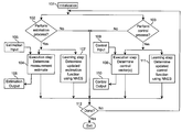
- FIG. 1 is a block diagram showing the major steps taken in performing estimation and/or control in accordance with the teachings of the present invention
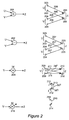
- FIG. 2 illustrates several types of circuit elements and the corresponding arrangements of nodes and connections in an ANN
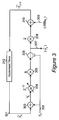
- FIG. 3 illustrates a circuit and data flow for performing an estimation process and for learning an optimal estimation function
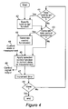
- FIG. 4 is a flow diagram showing the main elements of a system that learns and executes a control function
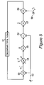
- FIG. 5 illustrates a circuit and data flow for learning an optimal control function
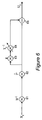
- FIG. 6 illustrates a circuit and data flow for calculating a control output signal given a learned control function
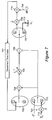
- FIG. 7 illustrates a circuit and data flow that combines the functions of learning and executing a control function
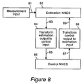
- FIG. 8 is a block diagram that illustrates the combination of estimation and control processes within a single system
- FIG. 9 illustrates an artificial neural network (ANN) flow diagram for optimal estimation, showing the flow of signal values, the nodes and connections of the neural network, connection weights, the computations that perform the execution process, and the computations that perform the learning process;
- ANN artificial neural network
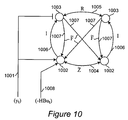
- FIG. 10 illustrates an ANN for optimal estimation, showing only nodes and connections, but not the detailed flow of signal values at each time;
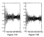
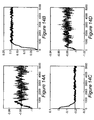
- FIGS. 11A and 11B are graphs showing the difference between the a posteriori plant state estimate computed from the output of an ANN according to the present invention, and the corresponding estimate computed using the classical Kalman estimation equations, for each of two vector components;
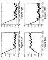
- FIGS. 12A, 12B , 12 C, and 12 D are graphs showing the neurally learned values (computed by an ANN) of an estimation function (I ⁇ HK t ) vs. time, and the solution using the classical Kalman estimation equations;
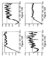
- FIGS. 13A, 13B , 13 C, and 13 D are graphs showing the neurally learned values of the Kalman filter K t vs. time, and the solution using the classical Kalman estimation equations;
- FIGS. 14A, 14B , 14 C, and 14 D are graphs showing the neurally learned values of a matrix, ( ⁇ tilde over (F) ⁇ t ), that describes the combined effect of the plant dynamics and the measurement process, and the (constant) known value of the quantity ( ⁇ HFH ⁇ 1 ), to which it converges.
- FIG. 1 is a block diagram showing the major steps taken in performing estimation and/or control in accordance with the teachings of the present invention.
- the estimation and/or control processes are initialized. If an estimation process is to be performed, this initialization comprises specifying an estimation error criterion, a class of allowed estimation functions, and an initial estimation function selected from the class of allowed estimation functions. If a control process is to be performed, this initialization comprises specifying a control cost criterion, a class of allowed control functions, and an initial control function selected from the class of allowed control functions. Steps 102 and 103 may be performed sequentially in either order, or in parallel. At step 102 , it is determined whether an estimation process is to be performed. If it is, then steps 104 and 107 are performed.
- a measurement estimate is determined using a specified or previously determined estimation function (from step 101 or 107 ), and input provided by step 105 .
- This input comprises at least one measurement vector, and (if the control process is also being performed) a control vector that is provided as output at step 110 below.
- the measurement estimate is provided as output at step 106 .
- Step 107 determines an updated estimation function using a neural network equivalent system (NNES, defined below) and a previously specified or determined estimation function.
- NNES neural network equivalent system
- Step 103 it is determined whether a control process is to be performed. If it is, then steps 108 and 111 are performed. These steps may be performed sequentially in either order, or in parallel.
- a control vector is determined using a specified or previously determined control function (from step 101 or 111 ), and input provided by step 109 . This input comprises at least one of a plant state vector, a measurement vector, and a measurement estimate. A measurement estimate is available as the output of step 106 , if the estimation process is also being performed.
- the control vector is provided as output at step 110 .
- Step 111 determines an updated control function using a neural network equivalent system and a previously specified or determined control function.
- step 112 it is determined at step 112 whether a stopping condition has been satisfied; if it has not, a new iteration through the estimation and/or control processes commences at steps 102 and 103 . Note that if only the estimation (or, respectively, the control) process is to be performed, then it is unnecessary to repeat step 103 (or, respectively, step 102 ) at each iteration.
- ganging is only used for updating a covariance matrix using the “batch learning method” option described below in the section entitled “Updating a covariance matrix or inverse covariance matrix: neural network methods”. If one of the “incremental learning” methods described in that section is used instead, the ganging operation is not used.
- FIG. 2 shows (at the left) the circuit symbols used in this invention to indicate an operation, and (at the right) the ANN elements that perform that operation.
- the ANN elements are shown for. the case in which each vector has two components (shown as two nodes in the ANN); it is to be understood that one ANN node is to be used for each component of the vector that is being represented by the activities of the ANN nodes.
- H is an N y -by-N x rectangular vector, and has no inverse.
- the pseudoinverse H + should be used as a replacement for H ⁇ 1 ;
- the estimation system learns to produce measurement estimates. If one knows the values of the matrix H, one can derive the corresponding plant state estimates. Similarly, if H is available to the estimation system, the system can be used to generate plant state estimates.
- Equation 1 ⁇ circumflex over (F) ⁇ ′g ( I ⁇ T t ⁇ 1 g ) ⁇ circumflex over (F) ⁇ +B′rB+g.
- v t (k) Specify a method for choosing a plurality of activity vectors v t (k), indexed by a second index k.
- each v t (k) may be drawn at random in accordance with a specified probability distribution function.
- ⁇ circumflex over (M) ⁇ t+1 is a function of the previous set of strengths ⁇ circumflex over (M) ⁇ t and the set of vectors v t (k) that is indexed by k.
- v t+1 (k) g(v t (k), ⁇ circumflex over (M) ⁇ t ), where the function g can be implemented using neural computations.
- v t+1 ( k ) g ( v t ( k ), ⁇ circumflex over (M) ⁇ t ) ⁇ ⁇ ′[ ⁇ n t ( k )+ R ⁇ circumflex over (M) ⁇ t ⁇ 1 v t ( k )]+ B′m t ( k )+ n t+1 ( k ), (29) where n t (k) and m t (k) are random vectors, each independently drawn from a distribution having a mean of zero and the covariance matrix R (for n) or Q (for m) respectively.
- ⁇ circumflex over (M) ⁇ t+1 ⁇ ( ⁇ v t ( k ) ⁇ , ⁇ circumflex over (M) ⁇ t ) ⁇ v t ( k ) v′ t ( k )>, (30) where the angle brackets denote the mean over k.
- ⁇ circumflex over (M) ⁇ t+1 approximates Cov(v t ), with the approximation improving as the number of vectors indexed by k is increased.
- a key step in implementing estimation and/or control, using neural computations, is that of computing and updating the inverse of a covariance matrix.
- Equation 19 for estimation, or Equation 25 for control we have constructed a vector ( ⁇ t ⁇ for estimation, w t for control) whose covariance matrix inverse (Z t ⁇ 1 for estimation, T t ⁇ 1 for control) is involved in the computation of the corresponding vector at the next value of the time index (t+1 for estimation, t ⁇ 1 for control).
- NNES neural network equivalent system
- a covariance matrix is, by definition, the expectation value of the product of a vector and its transpose; for example, M ⁇ Cov(v) ⁇ E(vv′), where the mean value E(v) of v is zero.
- the expectation value E( . . . ) refers to an average over a distribution of vectors.
- v(k) the covariance matrix is approximated by ⁇ v(k)v′(k)>, where ⁇ . . . > denotes an average over k.
- the covariance matrix may be approximated by a running average over k in which, as each new v(k) is generated, the product term v(k)v′(k) is combined with a previous approximation of the covariance matrix.
- M ( k ) (1 ⁇ a ) M ( k ⁇ 1)+ av ( k ) v ′( k ) (31)
- M(k) denotes the running average through the k term
- a is a “learning rate” having a value between zero and one, which may either be kept constant or may be specified to vary with k (see “Use of Adjustable Learning Rates” below).
- a running average provides a sufficiently good approximation provided that the distribution is changing slowly enough.
- a set of connection strengths in an ANN corresponds to the values of a matrix ⁇ tilde over (M) ⁇ , which approximates the covariance matrix inverse M ⁇ 1 ; and the product ⁇ tilde over (M) ⁇ (k)v is then generated by neural computations.
- Incremental covariance learning This method is described in R. Linsker, Neural Computation, vol. 4 (1992), pp. 691-702, especially at pp. 694 and 700-701.
- the matrix D(k) is computed in a manner similar to the running average M(k) described above.
- the components of input vector v(k) correspond to the activities at the inputs of a set of nodes, at a time corresponding to index k. These nodes are interconnected by a set of lateral connections. Just prior to the kth update step, the lateral connection from node i to node j has strength M ji (k ⁇ 1).
- the input activity vector v to the nodes is held constant.
- this input v is passed through the lateral connections, so that v is thereby multiplied by the connection strength matrix D, and is fed back as input to the same set of nodes.
- the input activity vector v(k) is passed through the matrix of connections, yielding the activity vector ⁇ tilde over (M) ⁇ (k)v(k). Then an anti-Hebbian learning rule is used [it is called “anti-Hebbian” because of the minus sign on the last term, ⁇ az(k)z′(k)] to update the strengths ⁇ tilde over (M) ⁇ . Because the lateral connections are undirected, ⁇ tilde over (M) ⁇ (k) is a symmetric matrix. This is useful for technical reasons as described in the above-cited reference.
- D tnew is directly computed as an approximation of the identity matrix I minus a constant c times the covariance matrix of v. The approximation improves as the number of instances k is increased.
- connection strength matrix M ⁇ 1 v(k) is obtained by applying the input activity vector v(k) to the kth set of nodes, and iteratively passing the activities through the lateral connections D multiple times, as described above in the paragraph on “incremental covariance learning”.
- D tnew is computed by combining the previous matrix D t with the new quantity computed above, so that the updated matrix is intermediate between the D tnew of “replacement batch learning” and D t .
- D tnew (1 ⁇ a)D t +a ⁇ [I ⁇ cv(k)v′(k)]>. This method is useful when the number of sets k is insufficient to provide a sufficiently good approximation of I ⁇ cM (where M is the covariance matrix), so that a running average over successive times is desirable.
- Equation 31 above and learning rules to be discussed (see, e.g., Equations 35 and 38 below), involve numerical factors called learning rates (a, ⁇ Z , and ⁇ F in the referenced equations). These can be taken to be constant, as is done to obtain the results illustrated in the section entitled “Numerical Results” below. However, they can also be usefully adjusted during the learning process. Two purposes of this adjustment are to speed up the learning process, and to decrease the random fluctuations that occur in the weight matrices being learned.
- FIG. 12 As an example.
- the approach of that value to its final value is approximately linear. If the appropriate learning rate (in this case, ⁇ Z ) is increased, the slope of this approximately linear approach will also be increased in magnitude, resulting in a faster approach to the vicinity of the final value.
- the learned value is in the vicinity of its final value, it is desirable to decrease the value of the appropriate learning rate, in order to reduce the random fluctuations of the learned value about its correct value.
- the adjustments in the learning rate(s) can be specified explicitly, or can be made automatically.
- One way to make the adjustments automatically is to compare the size of the fluctuations in learned values, to the slope of the trend in those values. If the learned value is changing approximately linearly with time and fluctuations about this linear trend are relatively small, the learning rate should be kept relatively large or increased. Conversely, if fluctuations dominate the change in learned values, the learning rate should be kept relatively small or decreased.
- the task is to estimate the position of an object as a function of time, and the object has a plurality of identified features (e.g., visible markings) that are each tracked over time
- a separate measurement can be made of the position of each feature at each time step, and the measurement residual vector ⁇ t ⁇ an be computed for each such feature.
- this ensemble of measurement residual vectors can be used to compute an approximation, Z t , of the covariance matrix of ⁇ t ⁇ . This computation will be more accurate than that obtained by combining only a single value of the measurement residual vector with the computation of Z t ⁇ 1 , from the previous time step.
- economies of scale as well as increased speed can be realized by constructing a large number of sets of processors that, in parallel, process distinct parts of an input environment (e.g., a visual field) for estimation purposes, or generate and process independent vectors used in the learning of a control function (as described below), and combine the results of their computations in order to perform batch learning of a covariance matrix or covariance matrix inverse.
- an input environment e.g., a visual field
- a control function as described below
- FIG. 3 is a circuit showing the data flow in an embodiment of a neural network equivalent system for performing Kalman estimation.
- the circuit may be implemented in the form of special-purpose hardware or as a software program running on a general-purpose computer. If implemented as hardware, the circuit may be constructed from units that perform vector addition, multiplication of a vector by a matrix, and the other functions described above in the section entitled “Definition of Terms Relating to ANNs”, or the circuit may be implemented as a hardware ANN with nodes and connections as also described above.
- the circuit of FIG. 3 operates as follows.
- the measurement vector at time t, denoted y t is provided as input to the circuit by line 302 .
- This vector is multiplied by the matrix Z t ⁇ 1 at element 304 .
- a matrix updating process is carried out using one of the methods described above, in the section entitled “Updating a Covariance Matrix or Inverse Covariance Matrix: Neural Network Methods”.
- the values of either the matrix (I ⁇ cZ,) or Z t ⁇ 1 are updated (depending upon which matrix is being stored for use at the next time step, as discussed in the previous section), using the input ⁇ t ⁇ at element 304 to yield. the new matrix (I ⁇ cZ t+1 ) or Z t+1 ⁇ 1 respectively.
- the new matrix is stored for use by block 304 at the next time step t+1.
- the output of block 304 is then multiplied by R at block 305 , to yield output (RZ t ⁇ 1 ⁇ t ⁇ ).
- the measurement input from line 302 is subtracted from the output of block 305 .
- the output of block 306 is provided as the output vector from the circuit. This vector equals the negative of the a posteriori measurement estimate, ( ⁇ t ), by virtue of Equation 20 above.
- the quantity ( ⁇ t ) is also passed as input to element 308 , where it is multiplied by the matrix ⁇ tilde over (F) ⁇ .
- the result is added, at element 310 , to the vector denoted ( ⁇ HBu t ) that is provided as input on line 309 .
- the result, on line 311 is ( ⁇ t+1 ⁇ ), which is the negative of the a priori measurement estimate at time t+1.
- This result is provided as input to time delay element 312 , where the time step is incremented by one unit. Accordingly, the time step designated as t+1 at the input to element 312 is designated as t at the output from that element.
- the cycle then repeats for the new time step.
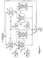
- FIG. 4 illustrates the general control process.
- step 41 it is determined whether a new cost-to-go function is to be provided. (The first time through the process, such a function must be provided. Thereafter, a new cost-to-go function may be provided when, e.g., the target state to be reached or approached changes, or when the nature of any of the contributing costs has changed.) If the answer is “yes”, then the new cost-to-go function is specified at step 42 .
- step 43 it is determined whether at least one new control function is to be generated. If the answer is “yes”, or if the process loop is being executed for the first time, then the new control function(s) is generated at step 44 .
- a selected control function is applied to the current plant state or measurement vector 48 .
- a possible reason for generating more than one control function at step 44 is so that a different one of the generated functions can be selected at step 45 during each of several different time steps, without having to re-enter step 44 at each new time step.
- Each such control function takes as an input the current plant state or measurement vector, and generates as an output a control output signal vector.
- the control output signal vector 46 is provided as output to the external plant, whereby it influences the future plant state, and is also optionally provided as output to other parts of the system, where it can be used, e.g., to influence the estimation of the plant state or the computation of a measurement estimate as described above.
- the time is then incremented at step 47 and if the control process is not yet completed (step 49 ), the process loop continues with step 41 .
- FIG. 5 shows a circuit for the learning of an optimal, or approximately optimal, control function.
- the flow process loop starting arbitrarily at block 51 . (The initialization of the process will be discussed later.)
- a random vector v t g is generated and passed along line 52 , to elements 53 and 56 .
- this vector is added to the result vector from the previous loop. The sum is equal to w t , the vector described by Equation 25.
- two events occur.
- the input to that step, w t is multiplied by the current value of T t ⁇ 1 , the inverse of the matrix T t , which is described by Equations 24 and 26.
- the current value of T t ⁇ 1 is updated to produce the value T t ⁇ 1 ⁇ 1 that will be used at the next execution of the loop (after the time index t has been decremented).
- the input vector to this block is multiplied by the matrix g.
- the random vector v t g is subtracted from the output of element 55 .
- the output of element 56 is the vector (gT t ⁇ 1 w t ⁇ v t g ).
- this vector is multiplied by the matrix ⁇ circumflex over (F) ⁇ ′.
- a random vector is computed by first drawing a random vector v t r from a distribution having zero mean and covariance matrix equal to r, and then multiplying this vector by the matrix B′.
- the vector denoted B′v t r may be generated as a random vector drawn from a distribution having zero mean and covariance matrix equal to B′rB.
- the outputs of element 57 and element 58 are added.
- the resulting vector is ⁇ circumflex over (F) ⁇ ′(gT t ⁇ 1 w t ⁇ v t g )+B′v t r .
- This vector is provided as input to element 51 , at which point the time index is decremented. by one. It is therefore seen that the vector w on the next execution of the loop, which is w t ⁇ 1 , is equal to the vector provided as input to block 51 , plus the new random vector v t ⁇ 1 g .
- the resulting expression for w t ⁇ 1 is identical to that given by Equation 25, showing that the circuit carries out the computation of w t ⁇ 1 as specified by that equation.
- a circuit that computes u t is given in FIG. 6 .
- the plant state vector x t is provided as input to the circuit at time t.
- x t is multiplied by the matrix B ⁇ 1 .
- the resulting vector is first multiplied by the matrix ⁇ circumflex over (F) ⁇ (element 62 ), then by matrix g (element 63 ), then by matrix T t ⁇ 1 (element 64 ).
- the modifiable matrix T t ⁇ 1 is the same matrix that was computed during the learning process, and stored either in the form T t ⁇ 1 or as (I ⁇ cT t ), as described above.
- the sum (T t ⁇ 1 g ⁇ I)( ⁇ circumflex over (F) ⁇ B ⁇ 1 x t ) is computed. This expression is equal to the desired optimal control output u t , as may be seen by comparing it with Equation 34.
- the control output u t influences the plant state x t+1 according to Equation 1. Note that u t is multiplied by matrix B to yield its contribution to x t+1 .
- FIG. 7 illustrates a combined circuit that performs both the learning function of the circuit of FIG. 5 , and the execution function of the circuit of FIG. 6 .
- the circuit operates in either of two modes, called “learning” (L) and “execution” (E) mode.
- the new tcurr has been advanced by one, and (in E mode) the corresponding input is applied and output is generated in turn.
- the mode is switched to L whenever a new control matrix needs to be computed; as noted above, this can be done every time tcurr advances by one, or an already-computed control matrix may be used (in the case that read-out and storage means are provided to preserve the values of the control matrix or matrices for values of the time index t>tcurr ).
- the matrix being learned and stored in this circuit, as connection strengths in a neural network implementation, is either (I ⁇ cT t ) or (T t ) ⁇ 1 , as described above; the quantity being used to compute either the next iteration (during L mode) or the control output vector u t (in E mode) is (T t ) ⁇ 1 , at element 75 .
- the “double-pole, triple-throw” switch (whose throws are shown as elements 702 , 707 , and 712 ) is set to the “up” position, marked “L”.
- the flow of signals through the circuit in L mode is as follows. At element 701 the time index is decremented by one. Output from that element passes through switch 702 , and a random vector v t g generated at element 703 passes through switch 712 . These two vector quantities are added together at element 704 . The result is multiplied by T t ⁇ 1 at element 705 .
- the values of the matrix (I ⁇ cT t ) or T t ⁇ 1 are also updated at element 705 .
- the same random vector v t g that was generated at element 703 is subtracted from the output of element 705 .
- the result passes through switch 707 , then is multiplied by ⁇ circumflex over (F) ⁇ ′ at element 708 .
- a random vector B′v t r is generated at element 709 , and the outputs from elements 708 and 709 are added at element 714 .
- the result is then passed to the time-decrementing element 701 .
- This entire sequence is the same as that already described for FIG. 5 , with the proviso that the matrix g has been eliminated (i.e., transformed into the identity matrix) as described above.
- the triple-throw switch is in the “down” position (marked “E”).
- the flow of signals through the circuit during this mode is as follows. Input ⁇ tilde over (x) ⁇ t from element 710 is multiplied by ⁇ circumflex over (F) ⁇ at element 711 , passes through switch 712 , and is applied as input to elements 704 and 706 . There is no other input to element 704 in this mode. The output from element 704 is multiplied by T t ⁇ 1 at element 705 (no learning or modification is performed at this block during E mode). The output of element 712 is subtracted from the output of element 705 at element 706 . The result passes through switch 707 and is provided as the output control signal u t at element 713 .
- the input to the control circuit is determined by a pre-processing step, in which ⁇ t is multiplied by H ⁇ 1 (see Equation 2) to obtain ⁇ circumflex over (x) ⁇ t , and the estimate ⁇ circumflex over (x) ⁇ t is then used in lieu of x t in the control circuit.
- ⁇ t is multiplied by B ⁇ 1 H ⁇ 1 to obtain the quantity that is then used in lieu of ⁇ tilde over (x) ⁇ t in the control circuit.
- FIG. 8 is a block diagram for combined optimal estimation and control.
- Block 82 performs an estimation process in which at least the learning step, and preferably the entire process, is performed by a neural network equivalent system.
- a preferred embodiment of this block is the circuit described by FIG. 3 .
- Block 86 performs a control process in which at least the learning step is performed by a neural network equivalent system.
- a preferred embodiment of this block is the circuit described by FIG. 7 .
- Measurement input is provided as input on line 81 , to the estimation block 82 .
- the output of that block provides information about the measurement estimate provided by block 82 .
- This output is transformed by block 84 to provide input, on line 85 , to control block 86 .
- the output of the control block on line 87 , provides information about the control signal generated by that block.
- This output is transformed by block 88 to provide input, on line 89 , to measurement block 82 .
- the entire cycle is repeated at a next time step.
- FIGS. 3 and 7 are used as embodiments of blocks 82 and 86 respectively, the vectors being transmitted and the transformations being performed in FIG. 8 are as follows:
- the measurement vector y t is provided as input on line 81 .
- the negative of the “a posteriori estimate at time t”, denoted ( ⁇ t ), is provided as output from the estimation block at line 83 . It is multiplied by the matrix ( ⁇ HB) ⁇ 1 at block 84 , to yield the vector ⁇ tilde over (x) ⁇ t at line 85 , which is provided as input to the control block 86 .
- the output of the control block is the control signal vector u t (on line 87 ), which is multiplied by the matrix ( ⁇ HB) at block 88 , and provided as input (line 89 ) to estimation circuit block 82 .
- ⁇ tilde over (x) ⁇ t (line 85 ) corresponds to line 710 of FIG. 7
- y t (line 81 ) corresponds to line 302 of FIG. E 2
- ( ⁇ t ) (line 83 ) corresponds to line 307 of FIG. 3
- ( ⁇ HBu t ) (line 89 ) corresponds to line 309 of FIG. 3 .
- FIG. 3 presented a circuit and data flow description of a neural network equivalent system (NNES) that performs Kalman optimal estimation. That description was given in terms of a sequence of neural computations to be performed, involving matrices and vectors.
- the neural computations can be implemented in hardware or software, as noted above with reference to the description of an NNES.
- a vector is implemented as a set of activity values over a set of nodes
- a matrix is implemented as a set of strengths of connections between a set of nodes and either the same set of nodes (in the case of “lateral” connections) or a different set of nodes.
- FIG. 9 describes an ANN implementation of the estimation process, in which (as also in the case of FIG. 3 ) both the learning and execution steps are performed by neural computations.
- FIG. 9 illustrates the learning of the matrices ⁇ tilde over (F) ⁇ and R.
- Those matrices were, for simplicity, treated as having been specified to the network in the case of FIG. 3 .
- FIG. 9 and the following description show how (a) optimal Kalman estimation, (b) the learning of the measurement noise covariance matrixt and (c) the learning of ⁇ tilde over (F) ⁇ , which is a problem in system identification, can all be performed by an NNES using only a stream of measurement vectors as inputs.
- the updating and use of the inverse covariance matrix Z t ⁇ 1 can be performed in an NNES by any of several methods.
- the “incremental covariance inverse learning” method is used.
- the other methods may be substituted for this if desired.
- the symbol ⁇ tilde over (Z) ⁇ denotes the matrix that is being updated to learn an approximation of the inverse covariance matrix Z ⁇ 1 , in similar fashion to the use of ⁇ tilde over (M) ⁇ in the above-referenced section.
- the flow diagram of FIG. 9 shows: the flow of signal values; the nodes and connections of a neural network; the connection weights, which are numerical values that in some cases are modified during processing; the computations that perform the execution process, by accepting input signal values and generating output signal values; and the computations that perform the learning process, by using the signal values at each end of a connection to modify the weight of that connection.
- the entire diagram shows the flow of information at one time step t of the measurement process.
- the processing takes place in several sequential “substeps” as one passes from the left to the right end of the diagram.
- Each of these substeps is called a “tick”.
- Each tick can correspond to one or more cycles in a conventional (clocked) computer or circuit. Alternatively, an unclocked circuit may be used provided that the results of various steps are each available at the required stage of the computation.
- the ticks are designated by lowercase letters a, b, . . . , j in alphabetical sequence.
- the next tick after tick j of time step t is tick a of time step t+1, and at this point one “wraps around” the diagram, from the right edge to the left, while incrementing the time from t to t+1.
- a plurality of neural network nodes is represented by two nodes denoted by circles, vertically disposed in the diagram. Circles that are horizontally disposed relative to each other denote the same node at different ticks. The tick letter is indicated inside each circle.
- the flow diagram is arranged in two “layers” denoted “Layer A” and “Layer B”. Thus two nodes in Layer A and two nodes in Layer B are indicated, each at several different ticks. There is no requirement that the nodes actually be disposed as geometric layers; the term “layer” here simply denotes that there are two distinct sets of nodes.
- connections between distinct nodes are represented by lines from one node at a given tick, to the other node at the next tick.
- the connections between each node and itself, or equivalently the processing that may take place within each individual node are represented by a horizontal line from each node at a given tick, to the same node at the next tick.
- Some of the lines are labeled by symbols; each such symbol either represents the value of the signal being carried on that line during that interval between adjacent ticks, or the connection weight by which the signal at the earlier tick is multiplied to obtain the signal at the next tick.
- a labeled double-line, drawn from one ordinary line to another ordinary line, represents a portion of the learning process, in which each connection weight denoted by the matrix symbol (which is drawn within a box) is modified by an amount that depends on the signal values on the ordinary lines between which the double-line is drawn.
- the signal values are denoted by symbols; for example, the new measurement at time t is denoted by y t .
- the measurement is a vector, or set of numerical values; in the neural network, each such value (i.e., each component of the vector) is provided as input to a distinct node.
- the notation is simplified by using the symbol for the vector, and so labeling a line to only one of the plurality of nodes.
- line 901 carries signal ( ⁇ t ⁇ ).
- the quantity ⁇ t ⁇ is called the “a priori estimate at time t”; i.e., the measurement estimate that the method of the present invention has computed for time t using only measurements available at time t ⁇ 1.
- Line 902 carries signal y t , the new measurement at time t.
- the two input signals are summed by each node 903 at tick a, producing on line 904 the signal ⁇ t ⁇ , called the “measurement residual”.
- tick b the signal value at each node is now multiplied by the weight of each connection that starts at that “source” node, and the signal values delivered by all of the connections that end at each “target” node are then summed.
- the rth source node at tick b carries the rth component of the vector ⁇ t ⁇ ; we denote this component by ( ⁇ t ⁇ ) r .
- the summed signal received at node s at tick c is given by ⁇ r ⁇ tilde over (Z) ⁇ t s ( ⁇ t ⁇ ) r .
- this sum is the sth element of the vector formed by the matrix product ⁇ tilde over (Z) ⁇ t ⁇ t ⁇ , which labels the lines 908 that emerge from the nodes at tick c.
- the set of nodes of Layer A at tick d (step 909 ) carry the signal values corresponding to the components of the matrix product ⁇ tilde over (Z) ⁇ t ⁇ t ⁇ .
- step 911 These signal values are transmitted unchanged along lines 910 to the nodes of layer B at tick e (step 911 ).
- the symbol I denotes the identity matrix, which leaves a vector of values unchanged.
- the signals at step 911 are matrix-multiplied by the matrix denoted R t , whose components are the weights of the connections 912 between the nodes of Layer B.
- the signal values of these nodes at tick ⁇ (step 913 ), and on its output lines 914 are therefore the components of the vector R t ⁇ tilde over (Z) ⁇ t ⁇ t ⁇ .
- the measurement y t (the same measurement as was provided as input along line 902 ) is provided again on line 915 as input to the nodes of layer B.
- the nodes of Layer B subtracts the respective components of y t from the inputs from lines 914 .
- the resulting output vector whose values are represented by the signals on lines 917 , is ( ⁇ t ).
- the vector ⁇ t is the “a posteriori estimate at time t”; i.e., the measurement estimate that the method of the present invention has computed for time t using the measurements available at time t including the new measurement y t .
- the quantity ( ⁇ t ) is the result of the estimation execution process, which has now combined the new measurement y t with a quantity (matrix product) derived from ⁇ t ⁇ , and thereby from y t and the a priori estimate ⁇ t ⁇ .
- the a priori estimate is in turn derived from the a posteriori estimate at the previous time step, thereby completing the estimation process of combining the current measurement with the estimate from a previous time step.
- the signal values corresponding to ( ⁇ t ) are conveyed to the nodes of Layer B at tick h (step 918 ). These values are provided as output along lines 924 . They are also matrix-multiplied (using the connections 919 that lead from Layer B to Layer A) by the matrix of weights ⁇ tilde over (F) ⁇ t , to yield signal values at the nodes of Layer A at tick i (step 920 ). If a control action or other external action, as designated by u t in Equation 1, is present, then it has an effect on the estimation process by contributing a set of input signal values, corresponding to the vector ( ⁇ HBu t ), at tick j (step 926 ).
- the output lines 921 from tick j carry the components of the vector ( ⁇ t+1 ⁇ ), which is the negative of the a priori estimate at the next time step t+1. These output lines are “wrapped around” as described above, to become lines 901 at the left edge of the diagram at the next time step. Since t is incremented by one, the vector denoted ( ⁇ t+1 ⁇ ) at line 921 is identical to the vector denoted ( ⁇ t ⁇ ) at line 901 . This completes the description of the execution process, except for the initialization of that process and the description of the “truncated mode” referred to above. We return to these later.
- step 922 between ticks c and d, and for each pair of Layer A nodes indexed by r and s, the values of the vector ( ⁇ tilde over (Z) ⁇ t ⁇ t ⁇ ) at nodes r and s are combined to yield a modification term. This modification term is then added to the weight ⁇ tilde over (Z) ⁇ t sr of the connection from node r to node s. This step constitutes the portion of the learning process that modifies ⁇ tilde over (Z) ⁇ t to yield ⁇ tilde over (Z) ⁇ t+1 .
- This learning rule is an example of “Incremental Covariance Inverse Learning” as discussed above in the section entitled “Updating a Covariance Matrix or Inverse Covariance Matrix: Neural Network Methods”. As discussed in that section, one may alternatively use a time-dependent learning rate ⁇ . Such a time-dependent rate may usefully be tuned both to increase convergence speed and to avoid divergence or excessive stochastic fluctuation of the matrix being learned.
- step 905 (the doubled line) appears on both the left and right hand sides of the diagram; this doubled line is understood to “wrap around” the diagram from the right to the left edge, corresponding to an operation that uses activity values computed at time t (after tick g ) and time t+1 (after tick a).
- step 905 for each node r of Layer B and each node s of Layer A, the value ( ⁇ t r ) at line 917 and the value ( ⁇ t ⁇ ) s at line 904 are combined to yield a modification term, which is then added to the weight ⁇ tilde over (F) ⁇ t sr of the connection 919 from node r to node s.
- the learning of ⁇ tilde over (F) ⁇ t occurs only when the system is not operating in truncated mode. It is understood that the layer-B activity present just before tick h of time step t persists unchanged until after tick a of time step t+1.
- connection weight matrix (denoted by R or R t ) that will represent an approximation of the covariance matrix of the measurement noise (also denoted by R), can be determined as follows. (1) If the measurement noise covariance matrix R is known, then the corresponding connection strength matrix may be directly set equal to R and remain unchanged thereafter (unless the measurement noise statistics themselves change with time). No R learning occurs in this case. (2) As has been described in prior art concerning the Kalman filter, one may turn off external input to the measurement sensors (we refer to this as “offline” operation), let the sensors run in this “offline” mode and generate sensor readings that are instances of the measurement noise alone, and use these readings to determine R.
- offline As has been described in prior art concerning the Kalman filter, one may turn off external input to the measurement sensors (we refer to this as “offline” operation), let the sensors run in this “offline” mode and generate sensor readings that are instances of the measurement noise alone, and use these readings to determine R.
- the sensor readings generated by this offline operation can be used within the neural network described above, to yield a strictly neural computation of R.
- the method is run in “truncated mode”, during which the neural circuit is temporarily cut at step 925 .
- the “measurement” input y t is simply an instance of the measurement noise process, which we denote as ⁇ t .
- the noise term ⁇ t has covariance R.
- FIG. 10 illustrates the physical elements of an ANN whose operation was described above in relation to FIG. 9 .
- FIG. 10 shows only the nodes and connections, but not the flow of the processing with time and from one tick to the next.
- Layers A and B are shown as the lower and upper layers of nodes, respectively. Of the plurality of nodes in each layer, two representative nodes are shown (horizontally disposed within each layer).
- Lines 1001 provide the components of input vector y t (the current measurement at time t) to the nodes 1002 of Layer A and also to the nodes 1003 of Layer B. These inputs to nodes 1003 are with negative sign, as indicated by the “T”-shaped terminator (as opposed to an arrow).
- the lateral (i.e., within-layer) connections 1004 between nodes of Layer A have weights corresponding to the matrix elements of ⁇ tilde over (Z) ⁇ t .
- the lateral connections 1005 between nodes of Layer B have weights corresponding to the matrix elements of R t .
- Each of these lateral connections may be implemented either as a single undirected connection, or as a pair of directed connections.
- the feed-forward connections 1006 from each node of Layer A to the corresponding node of Layer B have fixed weights of value one (denoted by the identity matrix I).
- the feedback connections 1007 from each node of Layer B to each node of Layer A have weights corresponding to the matrix elements of ⁇ tilde over (F) ⁇ t .
- the performance of the neural system shown in FIG. 9 is illustrated for a particular numerical case, using a two-dimensional dynamical system.
- the matrix F that describes the deterministic plant dynamics the matrix H that describes the deterministic relation between a plant vector and a measurement vector, the plant noise covariance matrix Q, and the measurement noise covariance matrix R, are not specified to the neural system.
- the matrix ⁇ tilde over (F) ⁇ HFH ⁇ 1 will be learned by the operation of the neural system, and this is the only combination of F and H that is required for the estimation process being performed.
- the matrix R will be learned by use of the “truncated mode” operation described above.
- the matrix Q will not need to be learned explicitly by the neural system, since it is not needed for the determination of either the estimation matrix (I ⁇ K t H) or of the measurement estimates according to the method of the present invention.
- the “incremental inverse covariance learning” method is used to learn the matrix Z ⁇ 1 .
- the a posteriori state estimate error, ⁇ t x t ⁇ circumflex over (x) ⁇ t , is a diagnostic measure of the performance of both the neural and the classical estimation method.
- ⁇ t x t ⁇ circumflex over (x) ⁇ t
- ⁇ t x t ⁇ circumflex over (x) ⁇ t
- FIGS. 11A and 11B shows the difference [ ⁇ t (clas) ⁇ t (neural)] vs. time, for each of the two vector components. That is, the vector that represents the a posteriori state estimate error computed using the neural circuit, is subtracted from the vector that represents the a posteriori state estimate error computed using the classical Kalman filter equations.
- the first component of this difference of two vectors is plotted in FIG. 11A as a function of time.
- the second component of this difference is plotted in FIG. 11B .
- FIGS. 12A, 12B , 12 C, and 12 D show the neurally learned values of (I ⁇ HK t ) vs. time, and the classical Kalman matrix solution.
- the 2 ⁇ 2 matrix components are shown in the subplots. That is, the (1,1) component of the neurally learned matrix (I ⁇ HK t ) is plotted versus time as the jagged line, and the same component of the classical Kalman matrix solution is shown as a horizontal line, in FIG. 12A ; the (1,2) components in FIG. 12B ; the (2,1) components in FIG. 12C ; and the (2,2) components in FIG. 12D .
- the jagged curves converge to the horizontal line in each case, then fluctuate around that line owing to the random character of the noise in the plant state and measurement processes.
- the ordinate axis scale differs for the various components, so that although the fluctuations appear visually to be large for the (2,1) component, for example, the magnitude of the fluctuations are only of the order of 0.01 (similar to that for the other components in this case).
- FIGS. 13A, 13B , 13 C, and 13 D show the neurally learned values of the Kalman filter K t (obtained from the (I ⁇ HK t ) results by using the known H) vs. time, and the classical Kalman matrix solution. The presentation is similar to that described in FIG. 12 .
- FIGS. 14A, 14B , 14 C, and 14 D show the neurally learned values of ( ⁇ tilde over (F) ⁇ t ) vs. time, and the exact values of ( ⁇ HFH ⁇ 1 ), shown as a horizontal line in each figure part.
- the exact values are known from our specification of the plant dynamics above, but have not been specified to the neural system. Note that the neurally learned values converge to the horizontal line in each case (apart from small random fluctuations). The presentation is similar to that described in FIG. 12 .
Landscapes
- Engineering & Computer Science (AREA)
- Artificial Intelligence (AREA)
- Evolutionary Computation (AREA)
- Physics & Mathematics (AREA)
- Health & Medical Sciences (AREA)
- Software Systems (AREA)
- General Physics & Mathematics (AREA)
- Theoretical Computer Science (AREA)
- Computer Vision & Pattern Recognition (AREA)
- Medical Informatics (AREA)
- Automation & Control Theory (AREA)
- Life Sciences & Earth Sciences (AREA)
- Biophysics (AREA)
- Computational Linguistics (AREA)
- Data Mining & Analysis (AREA)
- General Health & Medical Sciences (AREA)
- Molecular Biology (AREA)
- Computing Systems (AREA)
- General Engineering & Computer Science (AREA)
- Mathematical Physics (AREA)
- Biomedical Technology (AREA)
- Feedback Control In General (AREA)
Abstract
Description
- 1. Field of the Invention
- The present invention generally relates to neural networks, and more particularly, to recurrent neural networks for estimation (including prediction) and/or control.
- 2. Background Description
- This invention is concerned with the problems of optimal, or approximately optimal, estimation and control. In a standard formulation of these problems, there is an external system or “plant” described at each of a plurality of times by a plant state that evolves over time according to a stochastic plant process, and there is a stochastic measurement process that produces measurements at each of a plurality of times. The optimal estimation problem consists of using the measurements to generate estimates of the plant states over time, so as to minimize a specified measure of the error between the estimated and actual plant states. The term “estimation” can refer to prediction, filtering, and/or smoothing, as described below.
- The optimal control problem consists of using the measurements, or estimates thereof, to generate control signals that have the effect of altering the plant state in such a manner as to minimize a specified measure of the error between the actual and a specified desired (or target) plant state at one or more future times. A function, called the “cost-to-go”, is typically specified. This function describes the cost of a process that generates and applies a succession of control signals to the plant, resulting in a succession of plant states over time. Given the current plant state or an estimate thereof, or a measurement vector that conveys information about the plant state, it is desired to generate a sequence of control signal outputs such that the cost-to-go is substantially minimized. The cost is typically a combination of terms that reflect the cost of generating control output actions, and the cost (or benefit, with a minus sign applied) of the plant state approaching or reaching a desired target state (or succession of such target states).
- A classical method for treating optimal estimation and control problems is the Kalman filter or extended Kalman filter. The Kalman filter (KF) was first described in R. E. Kalman, Trans. ASME, Series D, Journal of Basic Engineering, Vol. 82 (1960), pp. 35-45. It solves the problems of optimal estimation and control when the plant and measurement processes satisfy certain conditions of linearity. The KF method also assumes knowledge of several types of parameters. It assumes that the deterministic portions of both the plant evolution (over time) process, and the measurement process (giving the relationship between the plant state and the measurement vector), are known; and that the noise covariances of both the plant evolution and measurement processes are also known. When the linearity condition is not strictly satisfied, the extended Kalman filter method (EKF) can be used to generate a linearized approximation of the plant and measurement processes. The EKF may be iteratively applied to obtain a sequence of linearized approximations. When the parameters of the plant evolution and measurement processes are not known, one can use a separate computation, “system identification”, to determine or estimate these parameters.
- Kalman Optimal Estimation and Control
- The state of an external system (the “plant”) governed by linear dynamical equations is described by a vector xt, which evolves in discrete time according to
x t+1 =Fx t +Bu t +m t (1)
where the matrix F describes the noise-free evolution of x, m denotes an additive plant noise vector, u denotes an optional vector that may be generated as a control output signal by a controller system, and matrix B describes the effect of u on the plant state x. Sensors measure a linear function of the system state, with additive measurement noise n:
y t =Hx t +n t. (2)
In classical Kalman estimation (e.g., the above-cited reference), it is assumed that the matrices H and F are known, and that the covariance matrices Q=Cov(m) of the plant noise, and R=Cov(n) of the measurement noise, are also known. Here E( . . . ) denotes expectation value, Cov(z)≡E[(z−z )(z−z )′],z is the mean of z, the prime symbol denotes matrix transpose, I will denote the identity matrix, and n and m are assumed to have zero mean.
Kalman Estimation - The goal of the optimal estimation process is to generate an optimal estimate of xτ given a set of measurements {y1, y2, . . . , yt}. If τ is greater than, equal to, or less than t, the estimation process is referred to as prediction, filtering, or smoothing, respectively. An “optimal” estimate is one that minimizes a specified measure of the error between the estimated and the true plant state. Typically, this measure is the mean square error (MSE) of the estimated with respect to the true state.
- Further notation and definitions are as follows. The a priori state estimate is {circumflex over (x)}t −≡{circumflex over (x)}(t|y1, . . . , yt−1), where the right-hand side denotes the estimated value of xt given the values of {y1, . . . , yt−1}. The a posteriori state estimate is {circumflex over (x)}t≡{circumflex over (x)}(t|y1, . . . , yt−1). The expression
ηt −≡(yt−H{circumflex over (x)}t −) (3)
is called the measurement “innovation” or “residual”, and is the difference between the actual and predicted (in the case that τ=t+1) measurements at time t. The a priori and a posteriori state estimate errors are, respectively, ξt −=xt−{circumflex over (x)}t − and ξt=xt−{circumflex over (x)}t, and the covariances of these respective errors are pt −=Cov(ξt −) and pt=Cov(ξt). Since the estimation algorithm does not have access to the actual state xt, pt − and pt are not directly known. They are iteratively estimated by the algorithm below, starting from arbitrary initial values; these estimates at time t are denoted by (capital) Pt − and Pt respectively. - Kalman's solution for the optimal filter (i.e., the case τ=t) is then described by the following procedure: Given arbitrary initial values for {circumflex over (x)}0 and P0 (P0 is however typically initialized to be a symmetric positive-definite matrix), iteratively compute for t=1, 2, . . . :
{circumflex over (x)} t − =F{circumflex over (x)} t−1 +Bu t−1 (4)
P t − =FP t−1 F′+Q (5)
K t =P t − H′(HP t − H′+R)−1 (6)
{circumflex over (x)} t ={circumflex over (x)} t − +K tηt − ={circumflex over (x)} t − +K t(y t −H{circumflex over (x)} t −) (7)
P t=(I−K t H)P t −(I−K t H)′+K t RK′ t. (8) - Combining Eqs. 5 and 8 yields
P t+1 − =FP t − F′+Q−FK t(HP t − H′+R)K′ t F′. (9)
This iterative solution may be regarded as consisting of two parts: an execution step during which a new estimate is computed (Eqs. 4 and 7) using an estimation function (here, Kt or (I−KtH), which are related to Pt −); and an updating step during which a new estimation function is generated (Eqs. 6 and 9) in terms of an estimation function at a previous time. - The solution for the optimal prediction problem with τ=t+1 is given by the same equations, using Eq. 4 to generate the optimal prediction {circumflex over (x)}t+1 − given measurements through time t.
- One extension of classical Kalman filtering, as noted above, is the extended Kalman filter (EKF) method. This can be used when the linearity conditions above are not strictly satisfied. EKF can be used to generate a linearized approximation of the plant and measurement processes, and may be iteratively applied to obtain a sequence of linearized approximations. The resulting solution is not strictly optimal in general, but only approximately so. The Kalman equations can also be generalized by allowing one or more of the matrices H, F, R, and Q to be functions of t. Also, when the parameters of the plant evolution and measurement processes are not known, one can perform a separate computation, “system identification”, to determine or estimate these parameters.
- Kalman Control
- We turn now to optimal Kalman control. The stochastic linear quadratic Gaussian (LQG) control problem can be described as follows, in the case of “full observability” (i.e., where the plant state vector xt at each time is assumed known). From a current plant state xtcurr at time tcurr<N, it is desired to optimize a set of control output signals {utcurr, utcurr+1, . . . , uN−1}. The trajectory of the plant state—that is, the sequence of states {xtcurr+1, . . . , xN}—will depend on the choice of the u values, on the initial state xtcurr, and on the noise terms {mtcurr, . . . , mN−1}.
- The quantity to be optimized is called the “cost-to-go”, and has the following form. The cost-to-go of the trajectory comprises a control-action cost u′tgut and a target-deviation cost x′trxt for each time step t from tcurr to N, where both g and r are specified symmetric positive-definite matrices. Thus the cost-to-go, denoted J, is
J=Σ t=tcurr N−1(u′t gu t +x′ t rx t)+x′N rx N. (10) - The optimization problem consists of determining the set of values of u for which the value of J, averaged over initial position xtcurr and plant noise, is a minimum. The solution has the form ut=−Ltxt, where L is the Kalman control matrix at time t.
- In one extension of the above formulation, at least one of the matrices g and r may be functions of t. Also, the cost-to-go function may include additional cross-terms involving both x and u. See, for example, the University of Lund (Sweden) online lecture notes at http://www.control.lth.se/˜kursdr/lectures/fl3LQsynth.pdf. Also, the cost-to-go may be described in terms of a desired target state xtarg, in which case each xt in Equation 10 should be replaced by xt−xtarg. In that case, the target state may itself vary with time, as for example in the case that the goal is to generate control signals so that the plant state xt may approximately follow a desired target trajectory.
- In certain special cases, the cost-to-go may be formulated in such a way that the optimal matrices Lt are independent of time. This is referred to as a “stationary” optimal control problem. In one such case, the final time t=N is considered to be effectively infinite. In another such case [see, e.g., Szita and Lörincz, Neural Computation, vol. 16 (2004), pp. 491-499], the final time t=N is considered to be indeterminate; i.e., if the cost-to-go terms have not terminated by an arbitrary time step t, they are assumed to terminate at the next time step t+1 with a given constant probability.
- For the optimal control problem stated above, the classical Kalman solution is described by the following procedure, where S is an auxiliary matrix that is a function of t. Starting with SN=r, iteratively compute for the decreasing sequence of time index values t=N, N−1, . . . , tcurr:
L t=(B′S t B+g)−1 B′S t F (11)
S t−1 =F′S t F+r−L′ t(B′S t B+g)Lt. (12)
Then, for t=tcurr and (optionally) for later t, use the Kalman Lt matrices to compute the control vectors ut:
u t =−L t x t (13) - This process generates the set of optimal control output vectors {utcurr, . . . , uN−1}. As in the case of estimation, but with a key difference (regarding the order of computation of functions having different values of the time index), this iterative solution may be regarded as consisting of two parts: an execution step during which a new control vector is computed (Eq. 13) using a control function (here, Lt, which is related to St); and an updating step during which a new control function is generated (Eqs. 11 and 12) in terms of a control function that is associated with a later time index.
- Note that, as observed by Kalman, the solutions to the optimal estimation and control problems are mathematically “dual” to one another.
Equations 11, 13, and 12 are related by this duality to Equations 6, 7, and 9 of the Kalman filter solution, respectively. As noted above, however, the S and L matrices of the control problem are iteratively computed from later to earlier time index values (i.e., “backward in time”), whereas the P− and K matrices of the filtering problem are computed “forward in time”. The Kalman filter matrix K can therefore be computed at time t and immediately applied to determine the optimal a posteriori state estimate {circumflex over (x)}t, whereas the Kalman control matrices Lt must first be computed for a sequence of decreasing time index values, before they can be applied at the current time t=tcurr and then at later times. - Artificial Neural Networks
- An artificial neural network (ANN) is characterized by processor nodes and connections between them, each node and connection typically being capable of performing only relatively simple computations, wherein the behavior of the nodes and connections is described by parameter values which either may be fixed or may be modifiable according to a specified learning or update rule. Some of the parameters describing the connections are referred to as connection “weights” or “strengths”. An ANN may be implemented either in hardware, or as software that is run on a general-purpose computer. A processor node is a computation unit (in hardware) or a simulation of such a unit (in software), wherein at least one input value is transformed into at least one output value. Typically the node computes, as its output, a specified function (which may be nonlinear) of the sum of its input values. Each input value or “activity” is typically described by a numerical value that may be time-varying. Time may be continuous-valued or may consist of discrete time steps. In a hardware implementation, an activity may be represented by any of a variety of signals, e.g., a level of, or change in level of, a current, voltage, or other physical quantity, wherein the magnitude, timing, and/or repetitive nature of the level or change carries the information. A processor node may be an internal node of the network (connected only to other nodes of the network), or may be a sensor or input node (providing or transducing information from the external environment to the network), or may be an effector or output node (generating signals from the network that influence the external environment).
- Each connection conveys an activity value from one processor to another. The connection may be passive (i.e., may just transmit the value unchanged from one processor to the other) or may be active (transform the value en route). In the latter case, the particular transformation is specified by at least one parameter. Typically the transformation consists of a simple multiplication of the activity value by the connection strength.
- Neural network computations are often described in terms of the behavior of a set of related nodes and connections. Suppose that there are two sets of nodes, one set of which (the source nodes) provides input to the other set (the target nodes). An activity vector, for example z=(z1, z2, . . . , zn), at a given time represents the fact that the activity at node k is equal to zk at that time. (Note that here the superscripts denote index values, not exponents.) A matrix C refers to a set of connections from source to target nodes, where Ckj is the strength of the connection from node j to node k. In the case that each target node simply computes the sum of its weighted inputs, then a target activity vector z is related to a source activity vector v by the matrix equation z=Cv, which represents the set of equations zk=ΣjCkjvj. If the kth target node computes a nonlinear function gk of the sum of its inputs, then we have instead zk=gk(ΣjCkjvj).
- In an ANN, connection weights may be “directed”, meaning that Cji and Cij correspond to different connections (from i to j and from j to i respectively), and (if both connections exist) have strengths that need not be equal; or “undirected”, meaning that the two strengths are required to be equal to each other.
- A layered ANN is one in which the nodes are organized into two or more groupings (called layers, but in the present invention not implying any particular geometric arrangement). Within a layered network, the connections may be within (a) a single layer (lateral connections), (b) from a “lower” to a “higher” layer in a hierarchy (feedforward connections), and/or (c) from a “higher” to a “lower” layer (feedback or recurrent connections). A layered ANN with recurrent connections is also called a recurrent neural network (RNN).
- Adjustable connection strengths, and other adjustable parameters, may be modified using a learning rule. Typically, a learning rule is “local”, meaning that the rule makes use only of activity values, connection strengths, and other parameters or state information that are available at the node or connection being modified. For example, a simple version of a “Hebbian” learning rule changes a strength Cji by an amount proportional to the product of the activities zi and zj at either end of the connection from i to j. In some cases, a learning rule may make use of certain global values or signals that are available at all, or a subset of, the nodes and connections. For example, in a “reinforcement learning” algorithm, the change in strength may be proportional to a quantity that represents the overall benefit or cost resulting from an output signal produced by the network at a previous time step.
- Also, in some cases, a subset of corresponding connections may be considered to be coupled or “ganged” together, so that they all have the same connection strength, and are all modified in tandem by the average of the amounts by which each such connection would have been modified if they were not so coupled. For one example of a network computation using ganged connections, see S. Becker and G. Hinton, Nature, vol. 355, pp. 161-163 (1992). This may be done either to speed up a computation (as in the above reference), or to cause corresponding parts of a network to behave in a coordinated manner.
- Other types of ANNs and learning rules have been described in the literature; for a good introduction, see J. Hertz, A. Krogh, and R. G. Palmer, Introduction to the Theory of Neural Computation, Addison-Wesley 1991. As one example, the information conveyed between nodes of an ANN may be carried by the precise timing of spikes (rapid changes in activity value) rather than by the numerical value of the activity itself. As a second example, another type of ANN is a “radial basis function” (RBF) network. The output of an RBF node decreases as a function of the distance between the set of inputs to the node (regarded as a vector) and a “prototype vector” that is stored as a set of parameters for that node; the prototype vector is typically modified according to an appropriate learning rule.
- Use of ANNs in Estimation and Control Problems
- Typically, an ANN is used to perform an estimation function (such as prediction) by a process of “supervised learning”, using a training set comprising both measurement values and the desired plant state values to be estimated. The network parameters (e.g., the connection strengths) are initialized, a set of measurement values is presented as input to the ANN, a set of output values is generated by the ANN, a measure of the error between the ANN's output and the desired output (the plant state at a given time) is computed, that error measure is used to modify the connection weights (and other adjustable parameters, if any) of the ANN according to a specified learning algorithm such as the “back-propagation” algorithm, and the process is iteratively repeated with a new set of inputs. The ANN's weights may thereby converge to values that cause the ANN to generate outputs whose error measure is sufficiently small.
- To treat the control problem, an ANN is typically used to generate one or more control outputs whose values depend upon the measurement inputs and the ANN's weights; the control outputs act on the plant (or on a simulated model of the plant) to alter the plant state; a measurement (or computation) of the new plant state is used as the new input to the network; and a measure of the error between the measured plant state and the target plant state is computed and used to modify the ANN's weights in accordance with a learning algorithm.
- Standard methods for training the weights of a recurrent neural network (RNN) based on time sequences of input values and desired output values include “real-time recurrent learning” and “back-propagation through time”, both of which are described in Hertzet al., ibid., pp. 182-186.
- J. T. Lo, in U.S. Pat. Nos. 5,963,929 and 5,408,424, describes the use of an RNN for optimal or near-optimal filtering (a form of estimation). In the '929 patent, a “recursive neurofilter” (RNN) is used to estimate a signal process with respect to an estimation error criterion, where at least one weight is a nonlinear weight and is adjusted during a separate training process. Also described is the use of a second “neurofilter” (a second circuit or algorithm), to produce an approximation of the statistical error of the estimates. In both the '929 and '424 patents, the neural network is trained using pairs of inputs—measurement data and the actual state of the plant—as discussed above. These pairs are used to train the connection strengths in a generic RNN (see col. 42 of the '424 patent specification). The patent relies on the general knowledge of “supervised learning” methods in the ANN field, regarding how to learn to match actual output with desired output, in order to train the weights. Note that information about the actual plant state is required for operation of this method. In practice, however, one may only have access to measurement data, and not to the plant state itself, preventing one from using this method. Note also that: the adjustable weights are kept fixed during operation of the network (that is, those weights are not being learned or adjusted while the filter is actually performing its estimation of a signal process); the second “neurofilter” is distinct from the first “neurofilter”; and although Kalman estimation is discussed as an alternative estimation method, Kalman estimation is not involved in the networks described (i.e., the networks neither learn nor use Kalman estimation).
- Neural networks have been used in conjunction with the Kalman estimation (also referred to as the Kalman filter, or KF) equations in several ways.
- First, the KF or EKF equations have been used to compute how the weights in an ANN should be modified. The ANN weights to be determined are treated as the unknown parameter values in a system identification problem, sets of input values and desired output values are specified, and the KF or EKF equations are used to determine the ANN weights based on the sets of input and desired-output values. The equations are solved by means of conventional mathematical steps including matrix multiplication and inversion. That is, the weights are not computed or updated (learned) by means of a neural network. Instead, the weights are read out from the neural network, provided as input arguments to the KF or EKF algorithm (which is not a neural network algorithm), the updated weight values are then provided as outputs of the KF or EKF algorithm, and the updated weight values are then entered into the neural network as the new weight values for the next step of the computation. For examples of this combined usage of an ANN in conjunction with the classical KF or EKF equations, see: S. Haykin (ed.), Kalman Filtering and Neural Networks, Wiley-Interscience, 2001, and in particular the chapter by G. V. Puskorius and L. A. Feldkamp; S. Singhal and L. Wu, “Training Multilayer Perceptrons with the Extended Kalman Algorithm”, in D. S. Touretzky (ed.), Advances in Neural Information Processing Systems, vol. 1 (Morgan Kaufmann Publ., San Mateo Calif., 1989), pp. 133-140; R. J. Williams, “Training recurrent networks using the extended Kalman filter”, in Proceedings of the International Joint Conference on Neural Networks, June, Baltimore, Md., Vol. IV (1992), pp. 241-246; and I. Rivals and L. Personnaz, “A recursive algorithm based on the extended Kalman filter for the training of feedforward neural models”, Neurocomputing, vol. 20 (1998), pp. 279-294.
- Second, one can combine the output from a nonlinear ANN with that of a (non-neural) KF algorithm, to improve predictions when applied to a nonlinear plant process. See for example Klimasauskas et al., “Hybrid linear—neural network process control”, U.S. Pat. Nos. 6,278,962 and 5,877,954. This method involves two analyzers: a primary “data-derived” one that generates a primary output, and a secondary “error correction analyzer” that generates a predicted error output; then the two analyzers' outputs are summed. Here the NN weights are trained to minimize the difference between (a) the sum of the linear filter output and the NN output, and (b) the desired output (e.g., the actual signal vector). That is, the NN learns how the linear filter output differs from the actual signal (or the desired output), and attempts to compensate for that difference. Here the NN does not learn a Kalman filter (KF); the KF is used alongside the NN, and the two perform complementary tasks. The KF is not computed or learned by means of a neural network or a set of neural computations. A similar combination is used in Tresp et al., “Method and arrangement for the neural modelling of a dynamic system with non-linear stochastic behavior”, U.S. Pat. No. 6,272,480. This method combines the output of a nonlinear recurrent neural network (RNN), with an error measure (based on a linear-equation model of the system error) that is modeled using a KF, in order to alter the RNN. The KF equations are not implemented within a neural network. They are solved, e.g., using a conventional computer program, and their values are then used to adjust the neural network's behavior.
- Third, an ANN learning rule has recently been described that is motivated by the KF equations, although it does not implement the learning of a KF within an ANN. See G. Szirtes, B. Póczos, and A. Lörincz, in Neurocomputing, vols. 65-66 (2005), pp. 349-355. In this method, the KF equations are first altered in several ways. One of these alterations replaces the matrix product HK, where H is as in Eq. 2 and K is the KF matrix, by the identity matrix I. This assumption that HK is approximately equal to I is, however, not valid in general, but only under special conditions. Another of these alterations neglects the off-diagonal terms in a matrix that is being updated. This alteration is stated to be justified when the estimated plant process satisfies an assumption of “independent component transformation”. For this assumption to hold, special preprocessing steps are in general required. Another alteration neglects a “self-excitatory” contribution. Yet another alteration introduces a random vector in order “to provide a conventional neuronal equation”, but this alteration incorrectly changes a significant term in the learning equation, so that the contribution of that term is averaged to zero. These alterations cause the resulting “learning rule” to fail to learn a KF matrix, even approximately. Furthermore, results displayed in that reference show a decreasing estimation error. However, the decrease shown is not the result of an approximation to a KF matrix having been learned. Similar results are obtained even when an arbitrary matrix K is used (instead of using an approximation to the KF matrix), with no learning at all taking place. For these reasons, this method does not implement the learning of a KF within an ANN.
- A classic formulation of the optimal control problem is Bellman's method of dynamic programming, in which (at each time step) a system has a set of allowed transitions from each state to a set of other states. A cost is associated with each transition, and the problem is to determine an optimal or near-optimal control policy that governs which transition to choose when in each state, to minimize an overall cost function. A class of ANN algorithms, based on “temporal difference” (TD) learning (a form of reinforcement learning) and its extensions, has been developed to learn the transition costs and a control policy. For a reference on TD learning (and reinforcement learning more generally) see: R. S. Sutton and A. G. Barto, Reinforcement Learning: An Introduction, MIT Press, 1998.
- For the more specialized case of a linear quadratic Gaussian (LQG) system, or for a linear quadratic (LQ) deterministic system, the optimal Kalman control (KC) solution is as discussed above. The general KC solution has not been implemented within an ANN. However, a solution of a particular specialized form of the LQG control problem, namely, the “stationary” optimal control problem discussed above, has been implemented using an ANN with a TD learning rule (Szita and Lörincz, loc. cit.). In this special case, as noted above, the cost-to-go terms are assumed to terminate at any future time step with a given constant probability.
- It is therefore an object of the invention to provide a method for estimation and/or control which involves a learning step and an execution step, wherein at least the learning step is performed by neural computations.
- A further object of the present invention is to provide a method for learning an optimal or near-optimal estimation and/or control function, in which the learning is performed by means of neural computations. These computations may be implemented within an artificial neural network, either in hardware or software form.
- A further object of the present invention is to integrate, within a single set of neural computations (e.g., a single ANN), (a) the learning of optimal or near-optimal estimation and/or control functions and (b) the execution of an estimation and/or control process using those learned functions, so that both the learning and execution can occur at the same time and using the same measurement input values.
- A further object of the present invention is to integrate, within a single set of neural computations (e.g., a single ANN), (a) the learning and use of an estimation and/or control function and (b) the learning and use of the required parameters describing the combined plant evolution and measurement processes (system identification), so that both steps (a) and (b) can occur at the same time and using the same measurement input values.
- A further object of the present invention is to perform optimal or near-optimal estimation and/or control by means of neural computations, in the case that only measurement values are available as input, and the actual plant state values are not known or available as input.
- A further object of the present invention is to perform optimal or near-optimal control, in the case that the “cost-to-go” function is not limited to the special case of a stationary optimal control problem.
- It is to be noted that the Kalman filter for estimation or control represents a special case of an estimation or control function.
- The present invention teaches the design of neural networks and neural network equivalent systems for optimal or approximately optimal estimation and/or control, including the design of a neural network architecture—a circuit with prescribed sets of connections between sets of nodes—and a set of learning rules that cause the circuit's connection strengths to evolve so as to learn optimal or approximately optimal estimation and/or control functions.
- According to one aspect of the present invention, there is provided a method for estimation which comprises the steps of (a) specifying an estimation error criterion, a class of allowed estimation functions, an initial estimation function selected from said class, and an initial measurement estimate, (b) inputting at least one measurement vector, (c) determining an updated estimation function using said estimation error criterion, a previously determined estimation function, a previous measurement estimate, and said at least one measurement vector, (d) determining an updated measurement estimate using an estimation function and said measurement vector, (e)outputting said updated measurement estimate, and (f) iterating steps (b) through (e) a plurality of times, wherein the step of determining an updated estimation function is performed using a neural network equivalent system (NNES).
- According to another aspect of the invention, there is provided a method for control, comprising the steps of (a) specifying a control cost criterion, a class of allowed control functions, and an initial control function selected from said class, (b) specifying a sequence of time values, (c) for each time value in said sequence of time values, determining an updated control function corresponding to said time value using said control cost criterion and a previously determined control function, (d) inputting state data comprising at least one of a plant state vector, a measurement vector, or a measurement estimate, (e) determining a control vector using one of said updated control functions and said state data, (f) outputting said control vector, (g) optionally iterating steps (d) through (f) one or more times, and (h) iterating steps (b) through (g) one or more times, wherein step (c) is performed using a neural network equivalent system (NNES).
- According to still another aspect of the invention, there is provided a neural network equivalent system (NNES) for estimation and/or control comprising a plurality of nodes connected to perform a sequence of steps in a prescribed order, said plurality of nodes comprising processors programmed or constructed to perform an execution step and/or a learning step using neural computations, input means for providing measurement values to said plurality of nodes, neural computation means for determining a plurality of measurement estimates, plant state estimates, and/or control vector signals using said measurement signals, and means for outputting said plurality of measurement estimates, plant state estimates, and/or control vector signals.
- The foregoing and other objects, aspects and advantages will be better understood from the following detailed description of a preferred embodiment of the invention with reference to the drawings, in which:
-
FIG. 1 is a block diagram showing the major steps taken in performing estimation and/or control in accordance with the teachings of the present invention; -
FIG. 2 illustrates several types of circuit elements and the corresponding arrangements of nodes and connections in an ANN; -
FIG. 3 illustrates a circuit and data flow for performing an estimation process and for learning an optimal estimation function; -
FIG. 4 is a flow diagram showing the main elements of a system that learns and executes a control function; -
FIG. 5 illustrates a circuit and data flow for learning an optimal control function; -
FIG. 6 illustrates a circuit and data flow for calculating a control output signal given a learned control function; -
FIG. 7 illustrates a circuit and data flow that combines the functions of learning and executing a control function; -
FIG. 8 is a block diagram that illustrates the combination of estimation and control processes within a single system; -
FIG. 9 illustrates an artificial neural network (ANN) flow diagram for optimal estimation, showing the flow of signal values, the nodes and connections of the neural network, connection weights, the computations that perform the execution process, and the computations that perform the learning process; -
FIG. 10 illustrates an ANN for optimal estimation, showing only nodes and connections, but not the detailed flow of signal values at each time; -
FIGS. 11A and 11B are graphs showing the difference between the a posteriori plant state estimate computed from the output of an ANN according to the present invention, and the corresponding estimate computed using the classical Kalman estimation equations, for each of two vector components; -
FIGS. 12A, 12B , 12C, and 12D are graphs showing the neurally learned values (computed by an ANN) of an estimation function (I−HKt) vs. time, and the solution using the classical Kalman estimation equations; -
FIGS. 13A, 13B , 13C, and 13D are graphs showing the neurally learned values of the Kalman filter Kt vs. time, and the solution using the classical Kalman estimation equations; and -
FIGS. 14A, 14B , 14C, and 14D are graphs showing the neurally learned values of a matrix, (−{tilde over (F)}t), that describes the combined effect of the plant dynamics and the measurement process, and the (constant) known value of the quantity (−HFH−1), to which it converges. -
FIG. 1 is a block diagram showing the major steps taken in performing estimation and/or control in accordance with the teachings of the present invention. Atstep 101, the estimation and/or control processes are initialized. If an estimation process is to be performed, this initialization comprises specifying an estimation error criterion, a class of allowed estimation functions, and an initial estimation function selected from the class of allowed estimation functions. If a control process is to be performed, this initialization comprises specifying a control cost criterion, a class of allowed control functions, and an initial control function selected from the class of allowed control functions.Steps step 102, it is determined whether an estimation process is to be performed. If it is, then steps 104 and 107 are performed. These steps may be performed sequentially in either order, or in parallel. Atstep 104, a measurement estimate is determined using a specified or previously determined estimation function (fromstep 101 or 107), and input provided bystep 105. This input comprises at least one measurement vector, and (if the control process is also being performed) a control vector that is provided as output atstep 110 below. The measurement estimate is provided as output atstep 106. Step 107 determines an updated estimation function using a neural network equivalent system (NNES, defined below) and a previously specified or determined estimation function. - At
step 103, it is determined whether a control process is to be performed. If it is, then steps 108 and 111 are performed. These steps may be performed sequentially in either order, or in parallel. Atstep 108, a control vector is determined using a specified or previously determined control function (fromstep 101 or 111), and input provided bystep 109. This input comprises at least one of a plant state vector, a measurement vector, and a measurement estimate. A measurement estimate is available as the output ofstep 106, if the estimation process is also being performed. The control vector is provided as output atstep 110. Step 111 determines an updated control function using a neural network equivalent system and a previously specified or determined control function. After the estimation and control processes have been carried out (or either of them has been bypassed), it is determined atstep 112 whether a stopping condition has been satisfied; if it has not, a new iteration through the estimation and/or control processes commences atsteps - We define the set of “elementary neural computations” to consist of the following mathematical operations:
-
- 1. Addition or subtraction of two vectors.
- 2. Multiplication of a vector by a matrix.
- 3. Transformation of a vector v into a vector z wherein each component zi of z is related to the corresponding component vi of v by the relationship zi=gi(vi) where gi is a mathematical function of one variable. The mathematical function may be fixed or adjustable.
- 4. Changing (updating) a function gi (as used above) to a new function {tilde over (g)}i that depends on the form of gi and the value of vi.
- 5. Changing (updating) the values of an adjustable matrix M, from M to {tilde over (M)}, wherein the matrix is associated with two vectors (that may be identical or distinct) v and z, and for each matrix component (j,i), {tilde over (M)}ji is a function of Mji, vi, and zj. The function may, but need not, depend on the values of i and j. One example of such an operation is the linear transformation
{tilde over (M)} ji=(1−α0)M ji+α1 v i z j+α2 v i+α3 z j+α4, - where {α0, . . . , α4} are specified numerical values; however, the definition is not limited by the scope of this example.
- 6. “Ganging” of corresponding pairs of vector values to update a matrix, meaning: Changing the values of an adjustable matrix M, from M to {tilde over (M)}, wherein: the matrix is associated with a plurality of pairs of vectors; the kth such pair is denoted by [v(k), z(k)]; the ith component of vector v(k) is denoted vi(k) (similarly for z); ƒji denotes a function of vi(k) and zj(k) that produces a numerical value as its output, and for each matrix component (j,i), {tilde over (M)}ji is a function of Mji and {ƒji(vi(k),zj(k))} for all k. One example of such an operation is the linear transformation
{tilde over (M)} ji=(1−α0)M ji+Σk[α1 v i(k)z j(k)+α2 v i(k)+α3 z j(k)]+α4, - where {α0, . . . , α4} are specified numerical values; however, the definition is not limited by the scope of this example.
Note that in general the participation or non-participation of a particular set of nodes in the ganging operation may change in accordance with other signals or the behavior of the network. For example, the sets of nodes that are ganged together may be determined by synchronous activity of nodes within and between those sets, as discussed further below. (However, in the specific embodiments described herein, the sets of nodes being ganged does not vary during operation of the network.) Also, a learning or update rule for connection strengths may use activity values over a range of times, rather than only at one time; this is true, for example, of “spike timing dependent” Hebbian learning rules.
- Also, in the embodiments described herein, ganging is only used for updating a covariance matrix using the “batch learning method” option described below in the section entitled “Updating a covariance matrix or inverse covariance matrix: neural network methods”. If one of the “incremental learning” methods described in that section is used instead, the ganging operation is not used.
-
- 7. Mode switching: Enabling the data flow, or flow of signals through a circuit, to be selected in accordance with a global signal that determines which of two or more modes is currently operative.
Each of the above elements corresponds in the following way to an element or set of elements within an ANN: A vector corresponds to a set of nodes, one node for each vector component. Both the node and its activity value may be denoted by a symbol of the form vi. A matrix M corresponds to the strengths (weights) of a set of connections, from a set of nodes corresponding to a vector v, to a set of nodes corresponding to a vector z. The sets of nodes may be two distinct sets, or they may be the same set. If they are the same set, the connections are referred to as “lateral” connections. [In the special case that M is a diagonal matrix (i.e., Mji≡0 for i not equal to j), the only connections required are from vi to zi for each i.] The connection strength from node vi to node zj is denoted by Mji. A node j, receiving connections of strengths Mji from each of a set of nodes i having activity values vi, respectively, produces as output the activity value zj=gj(ΣiMjivi). In the case of a “ganged” set of connections, the strength of each corresponding connection, from node i of set k (having activity value vi(k)) to node j of set k (having activity value zj(k)), has a value Mji that is the same for all k. The updating of Mji is likewise independent of k. Mode switching is accomplished either by the operation of one or more switches in a circuit, or by changes in the internal state of a set of nodes or connections.
- 7. Mode switching: Enabling the data flow, or flow of signals through a circuit, to be selected in accordance with a global signal that determines which of two or more modes is currently operative.
- Each of the operations described above corresponds in the following way to an operation within an ANN. For several of these operations,
FIG. 2 shows (at the left) the circuit symbols used in this invention to indicate an operation, and (at the right) the ANN elements that perform that operation. For simplicity, the ANN elements are shown for. the case in which each vector has two components (shown as two nodes in the ANN); it is to be understood that one ANN node is to be used for each component of the vector that is being represented by the activities of the ANN nodes. -
- 8. Addition or subtraction of two vectors (denoted by u and v) to produce a third vector z: Each output node zi receives connections from the two nodes ui and vi, and combines the input activities to form the sum zi=ui+vi or difference zi=ui−vi.
Circuit symbol 201 denotes this operation for addition, and 202 for subtraction. In the ANN representation,nodes connection 206 joins each of the two input nodes for each vector component to the corresponding output node for that vector component, in the case of addition.Connections 207 join the input nodes to the corresponding output nodes in the case of subtraction. The “T”-shaped termination, instead of an arrow, denotes the vector that is being subtracted (at element 202) or the connection whose activity is being subtracted (at element 207). - 9. Multiplication of a vector by a matrix: Each output node zj receives connections from nodes vi, each connection having strength Mji, and the total activity received by each node zj is the weighted sum ΣiMjivi.
Circuit symbol 208 denotes this operation. There are two ANN representations that correspond to this operation, depending upon whether (a) the nodes whose activities represent the output vector are a different set of nodes from those whose activities represent the input vector, or (b) the same set of nodes at a later time step. (a) In the first case,nodes connection 211 joins each input node to each output node. In general, if there are nv input nodes and nz output nodes, the number of connections is the product nvnz. (b) In the second case (showing “lateral” connections), the output activities z replace the input activities v after a time step or time interval has elapsed.Nodes 212 denote the ANN nodes in this case, andconnections 213 the connections from each node to each node. In general, all pairs of nodes may have a connection between them, including self-connections from a node to itself as shown. In practice, unneeded connections (those corresponding to matrix elements that are always zero) may be omitted. The connections may be directed (carrying activity in one direction only) or undirected (carrying activities in both directions). In the undirected case, the connection strengths in both directions are equal; i.e., Cji≡C ij for all pairs (i,j). The undirected case is denoted by the double-arrowedconnections 215 joiningnodes 214. - 10. Transformation according to zi=gi(vi): Here vi denotes the total input activity to node i, and zi the output activity.
- 11. Updating of a function gi: The change in the function gi depends only on information available at that node i; namely, the form of gi itself, and the activity vi at that node.
- 12. Updating of a connection strength matrix M: The change in each connection strength Mji depends only on information available at that connection and at the nodes it connects; namely, the values of Mji itself, and of the activities vi and zj. Circuit symbol 216 denotes this operation. In an ANN representation, as will be discussed below in connection with
FIG. 9 , components of the two activity vectors that are used to determine the modification of the connection strengths will be denoted by a double-line joining those components. - 13. “Ganging” to update a connection strength matrix: Here all corresponding connections (i.e., from a specified node i to a specified node j, within each set indexed by k) have the same strength Mji for all k. The ANN has a connection from node i to node j within each set k, and has communication means whereby corresponding connections maintain the same strength independent of k, and whereby the change in that common strength Mji (for each pair (i,j)) is determined by a set of contributions, one from each set k, with each contribution (for a given k) being computed using only information available at that connection (from node i to node j within that set k).
An example of the use of ganged connections is as follows. Consider a network in which there are multiple sets of source nodes (i;k) and of target nodes (j;k), wherein each set is designated by the index k and each node within a given set is designated by index i (for source node) or j (for target node). The connection from node i to node j within set k is denoted (j,i;k). At a given time, each such connection (in the absence of ganging) might be modified by an amount proportional to the product of the source and target activities within that group, i.e., zj(k)zi(k). As a result of the ganging, the connection strength Mji would be the same for all sets k, and would be modified by an amount proportional to the average of the products of corresponding activities, i.e., <zj(k)zi(k)>k where the angle brackets denote an average over the set index k. Various methods may be used to implement the ganging of connections. In a software implementation of such a network, a simple averaging (as above) may be performed. In a hardware implementation, the communication required to coordinate the behavior of corresponding portions of a network may be accomplished by other means including the precise timing (e.g., synchronization) of activity patterns in different parts of the network. Synchronization of activity patterns (including oscillations) has been described both in biological neural systems and in ANNs used to model aspects of perception and learning. Alternatively, in a hardware implementation, the activity vectors indexed by k may be communicated, one k value at a time, to a single processor complex that comprises the connection matrix C, thereby updating C. - 14. Mode switching: The flow or behavior of a set of activity signals or values, constituting an activity vector, is controlled by the mode switch operation. Examples of a change in the flow of activities is described below in relation to
FIG. 7 .
We define a “neural network equivalent system”, or “NNES”, to be a system selected from the group consisting of: - 15. An ANN implemented in hardware.
- 16. A software implementation of an ANN, run on a computer.
- 17. A circuit whose elements implement elementary neural computations.
- 18. A software program, run on a computer, whose steps implement elementary neural computations.
In the case of a hardware implementation of an ANN, or a circuit, the elementary neural computations may be performed either at discrete times or in a continuous fashion. In the latter case the ANN or circuit is preferably implemented using analog electronic computation means.
- 8. Addition or subtraction of two vectors (denoted by u and v) to produce a third vector z: Each output node zi receives connections from the two nodes ui and vi, and combines the input activities to form the sum zi=ui+vi or difference zi=ui−vi.
- Kalman Estimation
- We first consider the equations for classical Kalman estimation,
Equations 1 to 9. We define the auxiliary matrix
Z t =HP t − H′+R. (14)
Then Equation 6 yields
(I−HK t)=RZ t −. (15)
Using Equations 9 and 15, and defining {tilde over (F)}=HFH−1, we derive
Z t+1 ={tilde over (F)}(I−RZ t −1)R{tilde over (F)}′+HQH′+R. (16)
(Note: If the dimension Ny of a measurement vector y is less than the dimension Nx of a plant state vector x, then H is an Ny-by-Nx rectangular vector, and has no inverse. In this case the pseudoinverse H+ should be used as a replacement for H−1; the pseudoinverse is a standard generalization of the matrix inverse H−1, and is defined as H+=H′(HH′)−1. If one makes this replacement of H−1 by H+ in all equations, all of the results remain unchanged.) - Also, the measurement residual (defined above) equals
ηt − =y t −H{circumflex over (x)} t − =Hx t +n t −H{circumflex over (x)} t − =Hξ t − +n t, (17)
Pt −=Cov(ξt −), and R=Cov(nt), yielding
Cov(ηt −)=HP t − H′+R=Z t. (18)
The time evolution of η− is derived usingEquations
ηt+1 − ={tilde over (F)}RZ t −1ηt − −{tilde over (F)}n t +Hm t +n t+1. (19)
One can confirm algebraically that this equation implies Cov(ηt+1 −)=Zt+1, as it must since Equation 18 holds for all t. - We define the following quantities for later use: the a priori measurement estimate ŷt −≡H{circumflex over (x)}t −, and the a posteriori measurement estimate ŷt≡H{circumflex over (x)}t. Using Equations 3, 4, 7 and 15, we derive
ŷ t =y t −RZ t −1ηt − (20)
and
ŷ t+1 − ={tilde over (F)}ŷ t +HBu t. (21) - Note that the above equations have been expressed in a form that involves measurement estimates {tilde over (y)}t − and ŷt, and the matrix {tilde over (F)}, but does not explicitly involve the plant state xt, plant state estimates {circumflex over (x)}− and {circumflex over (x)}, or the matrices F and H (except through the term (HBut), which is provided as input to the estimation system). The system performing the estimation does not require, and in general may not have access to, knowledge of either the transformation H that relates plant states to measurements, nor of the plant evolution matrix F that determines how xt+1 is related to xt. Only the combination {tilde over (F)}≡HFH−1 is required, and that combination is learnable using measurements alone (as shown below in the section entitled “Detailed Example of ANN Implementation of Optimal Kalman Estimation”). Thus, the estimation system learns to produce measurement estimates. If one knows the values of the matrix H, one can derive the corresponding plant state estimates. Similarly, if H is available to the estimation system, the system can be used to generate plant state estimates.
- Kalman Control
- We now consider the Kalman control equations,
Equations
T t =B′S t B+g. (22)
ThenEquation 11 yields
I−B′(F′)−1 L′ t =gT t −1. (23)
Using Equations 12 and 23, and defining {circumflex over (F)}=B−1FB, we derive
T t−1 ={circumflex over (F)}′g(I−T t −1 g){circumflex over (F)}+B′rB+g. (24)
(Similarly to the note regarding H−1 above, if the dimension Nu of a control vector u is less than Nx, then B is an Nx-by-Nu rectangular matrix, and B−1 should be replaced throughout by the pseudo-inverse B+=(B′B)−1B′.] Now we introduce new vectors wt, vt r, and vt g at each time step. The vector vt r is defined to be randomly drawn from a distribution having mean zero and covariance r; similarly, vt g is defined to be randomly drawn from a distribution having mean zero and covariance g. Each vector is drawn independently of the other one, and independently of the random drawings at all other time steps. Each of these vectors may be regarded as an artificially generated “noise” term, not arising from the plant or the measurement process, but added for the purpose of the computational process. - The vector wt is initialized (at time t=N) as wN=vN g, and is defined to change in the following way as the time index t is decremented:
w t−1 ={circumflex over (F)}′(gT t −1 w t −v t g)+B′v t r +v t−1 g. (25)
Equation 25 and the initialization of w have been so constructed that, for all times t,
T t =Cov(w t). (26)
To derive this, note that Equation 25 implies E[wt(vg)′t]=E[vt g(vg)′t]=g; then use Equation 25 to express Cov(wt−1) in terms of Cov(wt). If it is true that Cov(wt)=Tt, then algebraic manipulation leads to the result Cov(wt−1)=Tt−1. Since the initialization ensures that Equation 26 holds for t=N, and since the equation holds for t−1. whenever it holds for t, it follows by mathematical induction that the equation holds for all t≦N. - The important result of this section is that, for both Kalman estimation and control, we have constructed a vector (ηt − for estimation, wt for control), such that the covariance of that vector at each t equals a matrix (Zt for estimation, Tt for control), and such that the evolution of that vector (from t to t+1 for estimation, from t to t−1 for control) yields the Kalman matrices (Kt for estimation, Lt for control) at each time step t.
- NNES Implementation of a More General Class of Matrix Equations
- The construction described above can be extended more generally, beyond the cases of Kalman estimation and control, as follows. In a variety of applications it is necessary to compute, for each of a plurality of iteration index values t, a new matrix Mt+1, given a matrix Mt, where Mt+1=h(Mt) and h is a specified function. In cases for which the following construction can be performed, this construction enables the M matrix computation to be performed by an NNES.
- Specify a method for choosing a plurality of activity vectors vt(k), indexed by a second index k. For example, each vt(k) may be drawn at random in accordance with a specified probability distribution function. Specify a functional relationship between a connection strength matrix {circumflex over (M)}t+1 and the set of vectors {vt(k)}: {circumflex over (M)}t+1=ƒ({vt(k)},{circumflex over (M)}t), where the function ƒ can be implemented, by neural computations, as a learning rule for the matrix of strengths M. The notation indicates that {circumflex over (M)}t+1 is a function of the previous set of strengths {circumflex over (M)}t and the set of vectors vt(k) that is indexed by k. Specify also an evolution equation of the form vt+1(k)=g(vt(k),{circumflex over (M)}t), where the function g can be implemented using neural computations. Choose g such that the matrix {circumflex over (M)}t+1, thus computed, is approximately equal to h({circumflex over (M)}t), where the approximation improves as the number of vectors vt(k) (at each t) is increased. When this property is satisfied, and {circumflex over (M)} is suitably initialized to equal or approximate the original matrix M, then the iterative process of neural computations will determine the evolution of the matrix {circumflex over (M)}t and the set of vectors vt(k) at a succession of iteration index values t, and {circumflex over (M)}t will continue to approximate the matrix Mt whose computation was required. To summarize, when the iteration index equals t, {circumflex over (M)}t and {vt(k)} determine {circumflex over (M)}t+1 via function ƒ, and they determine {vt+1(k)} via function g; then the iteration is repeated for iteration
index t+ 1. Thereby the result of a set of neural computations will be to carry out the desired computation of the matrix Mt to the required degree of approximation. - As an important special case of this more general formulation, we consider the algebraic Riccati equation
X t+1 =A′X t A+Q−A′X t B(B′X t B+R)−1 B′X t A. (27)
Both the Kalman estimation and Kalman control problems have equations of this form. To perform this iterative computation using a NNES, we define Mt≡B′XtB+R, and also define for notational convenience Â=B−1AB. Then the X equation yields an equation for the evolution of M:
M t+1 =h(M t)≡R+B′QB+Â′(I−RM t −1)RÂ, (28)
which is the equation to be solved. To do this using an NNES, we specify the activity vector evolution equation to be:
v t+1(k)=g(v t(k),{circumflex over (M)} t)≡Â′[−n t(k)+R{circumflex over (M)} t −1 v t(k)]+B′m t(k)+n t+1(k), (29)
where nt(k) and mt(k) are random vectors, each independently drawn from a distribution having a mean of zero and the covariance matrix R (for n) or Q (for m) respectively. We specify the function ƒ to be the function
{circumflex over (M)} t+1=ƒ({v t(k)},{circumflex over (M)}t)≡<v t(k)v′ t(k)>, (30)
where the angle brackets denote the mean over k. Thus {circumflex over (M)}t+1 approximates Cov(vt), with the approximation improving as the number of vectors indexed by k is increased. Algebraic computation of Cov(vt+1), using Equation 29 and the fact that E(vtn′t)=E(ntn′tt)=R, yields the same equation as Equation 28, but with {circumflex over (M)} replacing M. Therefore, an NNES that implements Equation 29 and the batch learning method of Equation 30, or a related incremental learning method, as discussed in the next section, will solve the Riccati Equation 28. - A key step in implementing estimation and/or control, using neural computations, is that of computing and updating the inverse of a covariance matrix. As shown above (see Equation 19 for estimation, or Equation 25 for control), we have constructed a vector (ηt − for estimation, wt for control) whose covariance matrix inverse (Zt −1 for estimation, Tt −1 for control) is involved in the computation of the corresponding vector at the next value of the time index (t+1 for estimation, t−1 for control). In this section we describe several methods for learning and updating a matrix that is a sufficiently good approximation to a covariance matrix inverse, by means of a neural network equivalent system (NNES).
- A covariance matrix is, by definition, the expectation value of the product of a vector and its transpose; for example, M≡Cov(v)≡E(vv′), where the mean value E(v) of v is zero. The expectation value E( . . . ) refers to an average over a distribution of vectors. In the NNES methods discussed here, only a finite number of instances, denoted by v(k), of the vector v are available. If all such instances are drawn from (that is, generated according to) the same distribution, then the covariance matrix is approximated by <v(k)v′(k)>, where < . . . > denotes an average over k. If, on the other hand, the distribution is changing as the instances are generated, then the covariance matrix may be approximated by a running average over k in which, as each new v(k) is generated, the product term v(k)v′(k) is combined with a previous approximation of the covariance matrix. For example,
M(k)=(1−a)M(k−1)+av(k)v′(k) (31)
where M(k) denotes the running average through the k term, and a is a “learning rate” having a value between zero and one, which may either be kept constant or may be specified to vary with k (see “Use of Adjustable Learning Rates” below). Such a running average provides a sufficiently good approximation provided that the distribution is changing slowly enough.
Incremental Learning Methods - In order to use an ANN to compute an approximation to the inverse M−1 of a covariance matrix M, we first consider methods in which a running average is used, and refer to these as “incremental learning” methods. In one such method (“incremental covariance learning”), a set of connection strengths in an ANN corresponds to the values of a matrix D(k) that is simply related to M(k) according to D(k)=I−cM(k), where M(k) approximates the covariance matrix M. The product M(k)−1v, which is used in the present invention, is then generated by neural computations as will be shown. In a second such method (“incremental inverse covariance learning”), a set of connection strengths in an ANN corresponds to the values of a matrix {tilde over (M)}, which approximates the covariance matrix inverse M−1; and the product {tilde over (M)}(k)v is then generated by neural computations.
- Incremental covariance learning: This method is described in R. Linsker, Neural Computation, vol. 4 (1992), pp. 691-702, especially at pp. 694 and 700-701. The matrix D(k) is computed in a manner similar to the running average M(k) described above. The components of input vector v(k) correspond to the activities at the inputs of a set of nodes, at a time corresponding to index k. These nodes are interconnected by a set of lateral connections. Just prior to the kth update step, the lateral connection from node i to node j has strength Mji(k−1). At the kth update step, the strengths are updated according to D(k)=aI+(1−a)D(k−1)−acv(k)v′(k), which is derived from Equation 31. Then a series of substeps is carried out. (The index k will be omitted here for notational simplicity.) The input activity vector v to the nodes is held constant. At the first substep, this input v is passed through the lateral connections, so that v is thereby multiplied by the connection strength matrix D, and is fed back as input to the same set of nodes. Thus the activity vector after the first substep is z1=v+Dv. At the second substep, this activity z1 is again multiplied by D, and added to the constant input v, so that the resulting activity vector is z2=v+Dz1=v+Dv+D2v where D2 denotes the square of the matrix D. Iteratively repeating this process, after the nth substep, the activity vector is
z n =v+Dv+D 2 v+ . . . +D n v=(I+D+D 2 + . . . +D n)V, (32)
where the superscripts denote powers of D. For a suitable choice of the constant c (as described in the above-cited reference), this series converges to (I−D)−1v, which equals (1/c)M(k)−1v. A finite number of iterations converges to a sufficiently good approximation to this asymptotic result. Thus the goal of computing an output activity M(k)−1v by neural computations is accomplished. - Incremental covariance inverse learning: This method is described in R. Linsker, Neural Networks, vol. 18 (2005), pp. 261-265. It is based on the classic Sherman-Woodbury-Morrison matrix identity, and the neural learning rule has the form
{tilde over (M)}(k+1)=(1+a){tilde over (M)}(k)−az(k)z′(k) (33)
where z(k)={tilde over (M)}(k)v(k). To implement this in a neural network, {tilde over (M)} is represented by the strengths of an undirected set of lateral connections. The input activity vector v(k) is passed through the matrix of connections, yielding the activity vector {tilde over (M)}(k)v(k). Then an anti-Hebbian learning rule is used [it is called “anti-Hebbian” because of the minus sign on the last term, −az(k)z′(k)] to update the strengths {tilde over (M)}. Because the lateral connections are undirected, {tilde over (M)}(k) is a symmetric matrix. This is useful for technical reasons as described in the above-cited reference. Since {tilde over (M)}(k) provides an approximation to M−1, the output activity vector {tilde over (M)}(k)v(k) approximates M−1v, as desired.
Batch Learning Methods - We next consider a method in which a set of instances v(k) of the vector v are available at a given time t, and can be used to update the matrix Dt=I−cM, (as defined above, in the paragraph on “incremental covariance learning”) to a new value Dtnew. This method is suitable for use with neural network equivalent systems in which the “ganging” operation described above is available. In this case, there is a separate set of nodes for each value of the index k. The input activity to node i of set k is vi(k). The lateral connection strength from node i to node j within each set k is Dji, and is independent. of k.
- In one method, which we call “replacement batch learning”, a new matrix of strengths Dtnew is computed at each time step, according to Dtnew=I−c<v(k)v′(k)> or, equivalently, Dtnew=<[I−cv(k)v′(k)]>, where the angle brackets denote an average over k and the “ganging” operation is used. Thus, Dtnew is directly computed as an approximation of the identity matrix I minus a constant c times the covariance matrix of v. The approximation improves as the number of instances k is increased. Using this connection strength matrix, the quantity M−1v(k) is obtained by applying the input activity vector v(k) to the kth set of nodes, and iteratively passing the activities through the lateral connections D multiple times, as described above in the paragraph on “incremental covariance learning”.
- In a variant, which we call “blended batch learning”, Dtnew is computed by combining the previous matrix Dt with the new quantity computed above, so that the updated matrix is intermediate between the Dtnew of “replacement batch learning” and Dt. For example, one may define Dtnew=(1−a)Dt+a<[I−cv(k)v′(k)]>. This method is useful when the number of sets k is insufficient to provide a sufficiently good approximation of I−cM (where M is the covariance matrix), so that a running average over successive times is desirable.
- Use of Adjustable Learning Rates
- Equation 31 above, and learning rules to be discussed (see, e.g., Equations 35 and 38 below), involve numerical factors called learning rates (a, γZ, and γF in the referenced equations). These can be taken to be constant, as is done to obtain the results illustrated in the section entitled “Numerical Results” below. However, they can also be usefully adjusted during the learning process. Two purposes of this adjustment are to speed up the learning process, and to decrease the random fluctuations that occur in the weight matrices being learned.
- Consider
FIG. 12 as an example. When one or more components of the matrix being learned has a value far from its final value (see, e.g.,FIG. 12A ), the approach of that value to its final value is approximately linear. If the appropriate learning rate (in this case, γZ) is increased, the slope of this approximately linear approach will also be increased in magnitude, resulting in a faster approach to the vicinity of the final value. On the other hand, once the learned value is in the vicinity of its final value, it is desirable to decrease the value of the appropriate learning rate, in order to reduce the random fluctuations of the learned value about its correct value. The adjustments in the learning rate(s) can be specified explicitly, or can be made automatically. One way to make the adjustments automatically is to compare the size of the fluctuations in learned values, to the slope of the trend in those values. If the learned value is changing approximately linearly with time and fluctuations about this linear trend are relatively small, the learning rate should be kept relatively large or increased. Conversely, if fluctuations dominate the change in learned values, the learning rate should be kept relatively small or decreased. - Population Averaging and “Ganging” of Connections
- In the section entitled “Definitions of Terms Relating to ANNs” above, and in the section above on “Batch Learning Methods”, a neural computation involving the “ganging” of connections was described and used. An example of the utility of this operation in an estimation and/or control process is as follows. In contrast to incremental learning methods that use only one vector at a time to update a covariance matrix or a covariance matrix inverse, the learning process can be performed more rapidly by using a plurality of values of the measurement residual vector at each time step. For example, if the task is to estimate the position of an object as a function of time, and the object has a plurality of identified features (e.g., visible markings) that are each tracked over time, then a separate measurement can be made of the position of each feature at each time step, and the measurement residual vector ηt − an be computed for each such feature. Then one can use this ensemble of measurement residual vectors to compute an approximation, Zt, of the covariance matrix of ηt −. This computation will be more accurate than that obtained by combining only a single value of the measurement residual vector with the computation of Zt−1, from the previous time step. Since the simultaneous computation for each feature will in general require a set of neurons devoted to representing the signals obtained for each feature, the total number of required neurons will in general be increased, but this can be justified by the resulting speedup of the learning of the filter Zt. In a software implementation of an NNES, this use of “ganging” or population averaging is well-suited to parallel computing methods. In a hardware implementation using a neural network or other special-purpose circuitry, economies of scale as well as increased speed can be realized by constructing a large number of sets of processors that, in parallel, process distinct parts of an input environment (e.g., a visual field) for estimation purposes, or generate and process independent vectors used in the learning of a control function (as described below), and combine the results of their computations in order to perform batch learning of a covariance matrix or covariance matrix inverse.
-
FIG. 3 is a circuit showing the data flow in an embodiment of a neural network equivalent system for performing Kalman estimation. The circuit may be implemented in the form of special-purpose hardware or as a software program running on a general-purpose computer. If implemented as hardware, the circuit may be constructed from units that perform vector addition, multiplication of a vector by a matrix, and the other functions described above in the section entitled “Definition of Terms Relating to ANNs”, or the circuit may be implemented as a hardware ANN with nodes and connections as also described above. - The circuit of
FIG. 3 operates as follows. The vector denoted (−ŷt −), which is the a priori measurement estimate at time t, is carried byline 301. The measurement vector at time t, denoted yt, is provided as input to the circuit byline 302. Atelement 303, yt is added to (−ŷt −) to yield ηt −=yt−ŷt −. This vector is multiplied by the matrix Zt −1 atelement 304. Also atelement 304, a matrix updating process is carried out using one of the methods described above, in the section entitled “Updating a Covariance Matrix or Inverse Covariance Matrix: Neural Network Methods”. In this manner, the values of either the matrix (I−cZ,) or Zt −1 are updated (depending upon which matrix is being stored for use at the next time step, as discussed in the previous section), using the input ηt − atelement 304 to yield. the new matrix (I−cZt+1) or Zt+1 −1 respectively. The new matrix is stored for use byblock 304 at the next timestep t+ 1. The output ofblock 304 is then multiplied by R atblock 305, to yield output (RZt −1ηt −). Atblock 306 the measurement input fromline 302 is subtracted from the output ofblock 305. The output ofblock 306 is provided as the output vector from the circuit. This vector equals the negative of the a posteriori measurement estimate, (−ŷt), by virtue of Equation 20 above. - The quantity (−ŷt) is also passed as input to
element 308, where it is multiplied by the matrix {tilde over (F)}. The result is added, atelement 310, to the vector denoted (−HBut) that is provided as input online 309. The result, on line 311, is (−ŷt+1 −), which is the negative of the a priori measurement estimate attime t+ 1. This result is provided as input totime delay element 312, where the time step is incremented by one unit. Accordingly, the time step designated as t+1 at the input toelement 312 is designated as t at the output from that element. The cycle then repeats for the new time step. -
FIG. 4 illustrates the general control process. Atstep 41 it is determined whether a new cost-to-go function is to be provided. (The first time through the process, such a function must be provided. Thereafter, a new cost-to-go function may be provided when, e.g., the target state to be reached or approached changes, or when the nature of any of the contributing costs has changed.) If the answer is “yes”, then the new cost-to-go function is specified atstep 42. Atstep 43 it is determined whether at least one new control function is to be generated. If the answer is “yes”, or if the process loop is being executed for the first time, then the new control function(s) is generated atstep 44. - At
step 45, a selected control function is applied to the current plant state ormeasurement vector 48. Note that a possible reason for generating more than one control function atstep 44, is so that a different one of the generated functions can be selected atstep 45 during each of several different time steps, without having to re-enterstep 44 at each new time step. Each such control function takes as an input the current plant state or measurement vector, and generates as an output a control output signal vector. (A “vector” here denotes simply a set of one or more numerical values.) - The control
output signal vector 46 is provided as output to the external plant, whereby it influences the future plant state, and is also optionally provided as output to other parts of the system, where it can be used, e.g., to influence the estimation of the plant state or the computation of a measurement estimate as described above. The time is then incremented atstep 47 and if the control process is not yet completed (step 49), the process loop continues withstep 41. - A particular, and important, special case of the control problem is that of optimal Kalman control, or the “linear quadratic Gaussian” control problem. This case is discussed below. Note that, in general, the matrix quantities discussed below that are for notational convenience and simplicity taken to be constant in time, may instead vary with time in a specified way. In this fashion, certain nonlinear processes can be modeled and an approximation to optimal control can be realized. (This modification is analogous to the “extended Kalman filter” formulation of the estimation problem, discussed above.)
- Learning of the Optimal Control Function
-
FIG. 5 shows a circuit for the learning of an optimal, or approximately optimal, control function. We first describe the flow process loop, starting arbitrarily atblock 51. (The initialization of the process will be discussed later.) Atelement 51 the time index is decreased by one unit, so that if the loop that has just been completed corresponded to, e.g., a time index of t=5, the next loop will have time index t=4. A random vector vt g is generated and passed alongline 52, toelements element 53 this vector is added to the result vector from the previous loop. The sum is equal to wt, the vector described by Equation 25. Atelement 54 two events occur. First, the input to that step, wt, is multiplied by the current value of Tt −1, the inverse of the matrix Tt, which is described by Equations 24 and 26. Second, the current value of Tt −1 is updated to produce the value Tt−1 −1 that will be used at the next execution of the loop (after the time index t has been decremented). For a description of several methods that may be used to accomplish both the updating of T−1 and the multiplication of wt by T−1, see the section above entitled “Updating a Covariance Matrix or Inverse Covariance Matrix: Neural Network Methods”. - At
element 55 the input vector to this block is multiplied by the matrix g. Atelement 56 the random vector vt g is subtracted from the output ofelement 55. The output ofelement 56 is the vector (gTt −1wt−vt g). Atelement 57 this vector is multiplied by the matrix {circumflex over (F)}′. At element 58 a random vector is computed by first drawing a random vector vt r from a distribution having zero mean and covariance matrix equal to r, and then multiplying this vector by the matrix B′. Alternatively, the vector denoted B′vt r may be generated as a random vector drawn from a distribution having zero mean and covariance matrix equal to B′rB. Atelement 59 the outputs ofelement 57 andelement 58 are added. The resulting vector is {circumflex over (F)}′(gTt −1wt−vt g)+B′vt r. This vector is provided as input toelement 51, at which point the time index is decremented. by one. It is therefore seen that the vector w on the next execution of the loop, which is wt−1, is equal to the vector provided as input to block 51, plus the new random vector vt−1 g. The resulting expression for wt−1 is identical to that given by Equation 25, showing that the circuit carries out the computation of wt−1 as specified by that equation. - Initialization and termination of the loop: The flow may be initialized by starting at any of several blocks, preferably by specifying an arbitrary vector wN (or a set {wN(k)} of such vectors, as described below) at time index t=N, and then either (a) using that vector or vectors to compute TN −1 as will be discussed, or (b) specifying an arbitrary symmetric positive-definite matrix TN or TN −1 to be used for the multiplication at
element 54. The loop for t=N then proceeds from that point. The loop can then be terminated after Ttcurr has been computed at time index t=tcurr. - Executing Control; Computing the Control Output Vector
- The optimal control vector is given by ut=−Ltxt. Combining Equation 23 with the definition of {circumflex over (F)} yields
L t=(I−T t −1 g){circumflex over (F)}B− 1 . (34)
A circuit that computes ut is given inFIG. 6 . The plant state vector xt is provided as input to the circuit at time t. Atelement 61, xt is multiplied by the matrix B−1. The resulting vector is first multiplied by the matrix {circumflex over (F)} (element 62), then by matrix g (element 63), then by matrix Tt −1 (element 64). The modifiable matrix Tt −1 is the same matrix that was computed during the learning process, and stored either in the form Tt −1 or as (I−cTt), as described above. Atelement 65, the sum (Tt −1g−I)({circumflex over (F)}B−1xt) is computed. This expression is equal to the desired optimal control output ut, as may be seen by comparing it with Equation 34. - The control output ut influences the plant state xt+1 according to
Equation 1. Note that ut is multiplied by matrix B to yield its contribution to xt+1. This transformation of the control signal into the effect But on the plant typically occurs as a result of the physical interaction between the control output signal and the plant. If, in addition, physical means are provided to transform the plant vector xt into the vector {tilde over (x)}t=B−1xt, then block 61 may be omitted, and the input xt replaced by {tilde over (x)}t. - Also, in certain cases it may be desirable to simplify the circuit of
FIG. 5 by eliminating element 55 (multiplication by matrix g). This can be done as follows. Since g is a symmetric and positive-definite matrix, it can be written in the form g=Λ′Λ (called a Cholesky decomposition; see, e.g., Numerical Recipes in C, W. H. Press et al., (Cambridge Univ. Press, 2nd ed., 1992), p. 96. If one replaces vector u by Λu, matrix B by BΛ−1, and matrix g by the identity matrix I, then the equations for the cost-to-go and for the dynamics are both unchanged. If these replacements are made, thenelement 55 is eliminated fromFIG. 5 , andelement 63 is eliminated fromFIG. 6 . - Combined Learning and Execution of Control
- With the above simplifications having been made,
FIG. 7 illustrates a combined circuit that performs both the learning function of the circuit ofFIG. 5 , and the execution function of the circuit ofFIG. 6 . The circuit operates in either of two modes, called “learning” (L) and “execution” (E) mode. During L mode, the time index starts at t=N and is decremented by one unit atblock 701 each time a loop is completed, until the loop terminates at t=tcurr. During E mode, input {tilde over (x)}t (see above) is applied to the circuit at time step t=tcurr, and output ut is generated. After one time step has passed, the new tcurr has been advanced by one, and (in E mode) the corresponding input is applied and output is generated in turn. The mode is switched to L whenever a new control matrix needs to be computed; as noted above, this can be done every time tcurr advances by one, or an already-computed control matrix may be used (in the case that read-out and storage means are provided to preserve the values of the control matrix or matrices for values of the time index t>tcurr ). The matrix being learned and stored in this circuit, as connection strengths in a neural network implementation, is either (I−cTt) or (Tt)−1, as described above; the quantity being used to compute either the next iteration (during L mode) or the control output vector ut (in E mode) is (Tt)−1, at element 75. - During L mode, the “double-pole, triple-throw” switch (whose throws are shown as
elements element 701 the time index is decremented by one. Output from that element passes throughswitch 702, and a random vector vt g generated atelement 703 passes throughswitch 712. These two vector quantities are added together atelement 704. The result is multiplied by Tt −1 atelement 705. The values of the matrix (I−cTt) or Tt −1 (depending on the implementation choice, described above in the section entitled “Updating a Covariance Matrix or Inverse Covariance Matrix: Neural Network Methods”) are also updated atelement 705. The same random vector vt g that was generated atelement 703 is subtracted from the output ofelement 705. The result passes throughswitch 707, then is multiplied by {circumflex over (F)}′ atelement 708. A random vector B′vt r is generated at element 709, and the outputs fromelements 708 and 709 are added atelement 714. The result is then passed to the time-decrementing element 701. This entire sequence is the same as that already described forFIG. 5 , with the proviso that the matrix g has been eliminated (i.e., transformed into the identity matrix) as described above. - During E mode, the triple-throw switch is in the “down” position (marked “E”). The flow of signals through the circuit during this mode is as follows. Input {tilde over (x)}t from
element 710 is multiplied by {circumflex over (F)} at element 711, passes throughswitch 712, and is applied as input toelements element 704 in this mode. The output fromelement 704 is multiplied by Tt −1 at element 705 (no learning or modification is performed at this block during E mode). The output ofelement 712 is subtracted from the output ofelement 705 atelement 706. The result passes throughswitch 707 and is provided as the output control signal ut atelement 713. - The above description of the control system considered, for simplicity, the situation in which the plant state was fully observable, so that the plant state xt (or {tilde over (x)}t) was used as input to the controller. However, in a more general situation xt is not itself directly known, but an estimate {tilde over (x)}t of it, or an estimation method such as that described earlier in this specification, is used to provide a measurement estimate ŷt.
- In the latter case the input to the control circuit is determined by a pre-processing step, in which ŷt is multiplied by H−1 (see Equation 2) to obtain {circumflex over (x)}t, and the estimate {circumflex over (x)}t is then used in lieu of xt in the control circuit. Alternatively, ŷt is multiplied by B−1H−1 to obtain the quantity that is then used in lieu of {tilde over (x)}t in the control circuit.
-
FIG. 8 is a block diagram for combined optimal estimation and control.Block 82 performs an estimation process in which at least the learning step, and preferably the entire process, is performed by a neural network equivalent system. A preferred embodiment of this block is the circuit described byFIG. 3 .Block 86 performs a control process in which at least the learning step is performed by a neural network equivalent system. A preferred embodiment of this block is the circuit described byFIG. 7 . - Measurement input is provided as input on
line 81, to theestimation block 82. The output of that block, online 83, provides information about the measurement estimate provided byblock 82. This output is transformed byblock 84 to provide input, online 85, to controlblock 86. The output of the control block, online 87, provides information about the control signal generated by that block. This output is transformed byblock 88 to provide input, online 89, tomeasurement block 82. The entire cycle is repeated at a next time step. - In the case that
FIGS. 3 and 7 are used as embodiments ofblocks FIG. 8 are as follows: The measurement vector yt is provided as input online 81. The negative of the “a posteriori estimate at time t”, denoted (−ŷt), is provided as output from the estimation block atline 83. It is multiplied by the matrix (−HB)−1 atblock 84, to yield the vector {tilde over (x)}t atline 85, which is provided as input to thecontrol block 86. The output of the control block is the control signal vector ut (on line 87), which is multiplied by the matrix (−HB) atblock 88, and provided as input (line 89) toestimation circuit block 82. Note in particular that: {tilde over (x)}t (line 85) corresponds to line 710 ofFIG. 7 ; yt (line 81) corresponds to line 302 of FIG. E2; (−ŷt) (line 83) corresponds to line 307 ofFIG. 3 ; and (−HBut) (line 89) corresponds to line 309 ofFIG. 3 . -
FIG. 3 , discussed above, presented a circuit and data flow description of a neural network equivalent system (NNES) that performs Kalman optimal estimation. That description was given in terms of a sequence of neural computations to be performed, involving matrices and vectors. The neural computations can be implemented in hardware or software, as noted above with reference to the description of an NNES. - When an NNES is implemented as an ANN, a vector is implemented as a set of activity values over a set of nodes, and a matrix is implemented as a set of strengths of connections between a set of nodes and either the same set of nodes (in the case of “lateral” connections) or a different set of nodes.
-
FIG. 9 describes an ANN implementation of the estimation process, in which (as also in the case ofFIG. 3 ) both the learning and execution steps are performed by neural computations. In addition,FIG. 9 illustrates the learning of the matrices {tilde over (F)} and R. (Those matrices were, for simplicity, treated as having been specified to the network in the case ofFIG. 3 .) ThusFIG. 9 and the following description show how (a) optimal Kalman estimation, (b) the learning of the measurement noise covariance matrixt and (c) the learning of {tilde over (F)}, which is a problem in system identification, can all be performed by an NNES using only a stream of measurement vectors as inputs. - As discussed above, in the section entitled “Updating a Covariance Matrix or Inverse Covariance Matrix: Neural Network Methods”, the updating and use of the inverse covariance matrix Zt −1, which corresponds to block 304 of
FIG. 3 , can be performed in an NNES by any of several methods. For the implementation described byFIG. 9 , the “incremental covariance inverse learning” method is used. However, the other methods may be substituted for this if desired. The symbol {tilde over (Z)} denotes the matrix that is being updated to learn an approximation of the inverse covariance matrix Z−1, in similar fashion to the use of {tilde over (M)} in the above-referenced section. - The flow diagram of
FIG. 9 shows: the flow of signal values; the nodes and connections of a neural network; the connection weights, which are numerical values that in some cases are modified during processing; the computations that perform the execution process, by accepting input signal values and generating output signal values; and the computations that perform the learning process, by using the signal values at each end of a connection to modify the weight of that connection. - The entire diagram shows the flow of information at one time step t of the measurement process. Thus, the processing takes place in several sequential “substeps” as one passes from the left to the right end of the diagram. Each of these substeps is called a “tick”. Each tick can correspond to one or more cycles in a conventional (clocked) computer or circuit. Alternatively, an unclocked circuit may be used provided that the results of various steps are each available at the required stage of the computation. The ticks are designated by lowercase letters a, b, . . . , j in alphabetical sequence. The next tick after tick j of time step t, is tick a of time step t+1, and at this point one “wraps around” the diagram, from the right edge to the left, while incrementing the time from t to t+1.
- A plurality of neural network nodes is represented by two nodes denoted by circles, vertically disposed in the diagram. Circles that are horizontally disposed relative to each other denote the same node at different ticks. The tick letter is indicated inside each circle. The flow diagram is arranged in two “layers” denoted “Layer A” and “Layer B”. Thus two nodes in Layer A and two nodes in Layer B are indicated, each at several different ticks. There is no requirement that the nodes actually be disposed as geometric layers; the term “layer” here simply denotes that there are two distinct sets of nodes.
- The connections between distinct nodes are represented by lines from one node at a given tick, to the other node at the next tick. The connections between each node and itself, or equivalently the processing that may take place within each individual node, are represented by a horizontal line from each node at a given tick, to the same node at the next tick. Some of the lines are labeled by symbols; each such symbol either represents the value of the signal being carried on that line during that interval between adjacent ticks, or the connection weight by which the signal at the earlier tick is multiplied to obtain the signal at the next tick. A labeled double-line, drawn from one ordinary line to another ordinary line, represents a portion of the learning process, in which each connection weight denoted by the matrix symbol (which is drawn within a box) is modified by an amount that depends on the signal values on the ordinary lines between which the double-line is drawn. The signal values are denoted by symbols; for example, the new measurement at time t is denoted by yt. Recall that the measurement is a vector, or set of numerical values; in the neural network, each such value (i.e., each component of the vector) is provided as input to a distinct node. In the diagram, the notation is simplified by using the symbol for the vector, and so labeling a line to only one of the plurality of nodes.
- We first describe the flow of the computations at some time index t for which the execution and learning processes are already underway. The initialization phase, as well as the so-called “truncation mode” referred to at
step 925, will be discussed later. Starting at the left edge of the diagram,line 901 carries signal (−ŷt −). The quantity ŷt − is called the “a priori estimate at time t”; i.e., the measurement estimate that the method of the present invention has computed for time t using only measurements available at time t−1.Line 902 carries signal yt, the new measurement at time t. The two input signals are summed by each node 903 at tick a, producing online 904 the signal ηt −, called the “measurement residual”. Continuing with the description of the execution process (and returning later to the learning process in which double-line 905 participates), we reach tick b atstep 906. The signal value at each node is now multiplied by the weight of each connection that starts at that “source” node, and the signal values delivered by all of the connections that end at each “target” node are then summed. Mathematically, the rth source node at tick b carries the rth component of the vector ηt −; we denote this component by (ηt −)r. The component of the weight matrix {tilde over (Z)}t that connects source node r to target node s, alonglines 907, is denoted by {tilde over (Z)}t sr. Then the summed signal received at node s at tick c is given by Σr{tilde over (Z)}t s(ηt −)r. In matrix notation, this sum is the sth element of the vector formed by the matrix product {tilde over (Z)}tηt −, which labels thelines 908 that emerge from the nodes at tick c. Thus the set of nodes of Layer A at tick d (step 909) carry the signal values corresponding to the components of the matrix product {tilde over (Z)}tηt −. - These signal values are transmitted unchanged along
lines 910 to the nodes of layer B at tick e (step 911). (The symbol I denotes the identity matrix, which leaves a vector of values unchanged.) The signals atstep 911 are matrix-multiplied by the matrix denoted Rt, whose components are the weights of theconnections 912 between the nodes of Layer B. The signal values of these nodes at tick ƒ (step 913), and on itsoutput lines 914, are therefore the components of the vector Rt{tilde over (Z)}tηt −. Next, the measurement yt (the same measurement as was provided as input along line 902) is provided again on line 915 as input to the nodes of layer B. At tick g (step 916) the nodes of Layer B subtracts the respective components of yt from the inputs fromlines 914. - The resulting output vector, whose values are represented by the signals on
lines 917, is (−ŷt). The vector ŷt is the “a posteriori estimate at time t”; i.e., the measurement estimate that the method of the present invention has computed for time t using the measurements available at time t including the new measurement yt. The quantity (−ŷt) is the result of the estimation execution process, which has now combined the new measurement yt with a quantity (matrix product) derived from ηt −, and thereby from yt and the a priori estimate ŷt −. We shall shortly see that the a priori estimate is in turn derived from the a posteriori estimate at the previous time step, thereby completing the estimation process of combining the current measurement with the estimate from a previous time step. - The signal values corresponding to (−ŷt) are conveyed to the nodes of Layer B at tick h (step 918). These values are provided as output along lines 924. They are also matrix-multiplied (using the
connections 919 that lead from Layer B to Layer A) by the matrix of weights {tilde over (F)}t, to yield signal values at the nodes of Layer A at tick i (step 920). If a control action or other external action, as designated by ut inEquation 1, is present, then it has an effect on the estimation process by contributing a set of input signal values, corresponding to the vector (−HBut), at tick j (step 926). Theoutput lines 921 from tick j carry the components of the vector (−ŷt+1 −), which is the negative of the a priori estimate at the next timestep t+ 1. These output lines are “wrapped around” as described above, to becomelines 901 at the left edge of the diagram at the next time step. Since t is incremented by one, the vector denoted (−ŷt+1 −) atline 921 is identical to the vector denoted (−ŷt −) atline 901. This completes the description of the execution process, except for the initialization of that process and the description of the “truncated mode” referred to above. We return to these later. - We next describe the learning process, again deferring a discussion of initialization. There are three sets of modifiable connection weights in this implementation. {tilde over (Z)}t, Rt, and {tilde over (F)}t. The role of the learning process is to cause: the weight matrix {tilde over (Z)}t to converge to Z−1 where Z is defined by Equation 14; the weight matrix Rt to converge to the measurement noise covariance matrix R which was defined following
Equation 2; and the weight matrix {tilde over (F)}t to converge to the matrix {tilde over (F)} defined following Equation 15. - Learning of Z: At
step 922, between ticks c and d, and for each pair of Layer A nodes indexed by r and s, the values of the vector ({tilde over (Z)}tηt −) at nodes r and s are combined to yield a modification term. This modification term is then added to the weight {tilde over (Z)}t sr of the connection from node r to node s. This step constitutes the portion of the learning process that modifies {tilde over (Z)}t to yield {tilde over (Z)}t+1. - Specifically, the learning rule used is:
{tilde over (Z)} t+1=(1+γZ){tilde over (Z)} t−γZ({tilde over (Z)} tηt −)({tilde over (Z)} tηt −)′, (35)
where γZ is a small positive learning rate (as are also the other learning rates γR and γF to be introduced below). This learning rule is an example of “Incremental Covariance Inverse Learning” as discussed above in the section entitled “Updating a Covariance Matrix or Inverse Covariance Matrix: Neural Network Methods”. As discussed in that section, one may alternatively use a time-dependent learning rate γ. Such a time-dependent rate may usefully be tuned both to increase convergence speed and to avoid divergence or excessive stochastic fluctuation of the matrix being learned. - Learning of {tilde over (F)}: Note that step 905 (the doubled line) appears on both the left and right hand sides of the diagram; this doubled line is understood to “wrap around” the diagram from the right to the left edge, corresponding to an operation that uses activity values computed at time t (after tick g ) and time t+1 (after tick a). At
step 905, for each node r of Layer B and each node s of Layer A, the value (−ŷt r) atline 917 and the value (ηt −)s atline 904 are combined to yield a modification term, which is then added to the weight {tilde over (F)}t sr of theconnection 919 from node r to node s. In this embodiment, the learning of {tilde over (F)}t occurs only when the system is not operating in truncated mode. It is understood that the layer-B activity present just before tick h of time step t persists unchanged until after tick a of timestep t+ 1. - To derive the specific learning rule for {tilde over (F)} in this implementation, we seek to minimize the mean square a priori measurement estimation error, which is MSE(ηt+1 −)≡E[(ηt+1 −)′(ηt+1 −)]. Using ŷt≡H{circumflex over (x)}t and
we find that the negative gradient of ½MSE(ηt+1 −) with respect to the elements of the matrix {tilde over (F)} is given by
The circuit implements stochastic gradient descent in {tilde over (F)} by using, instead of this expectation value, the current value of the matrix (ηt+1 −ŷ′t). This yields the learning rule for {tilde over (F)}:
{circumflex over (F)} t+1 ={tilde over (F)} t−γF(ηt+1 −)(−ŷ′t). (38)
This is an “anti-Hebbian” learning rule, since it decreases each connection weight by an amount proportional to the product of the activity (−ŷt)r at source node r times the activity (ηt+1 −)s at target node s. - Learning of R, and use of “truncated mode” operation: The connection weight matrix (denoted by R or Rt) that will represent an approximation of the covariance matrix of the measurement noise (also denoted by R), can be determined as follows. (1) If the measurement noise covariance matrix R is known, then the corresponding connection strength matrix may be directly set equal to R and remain unchanged thereafter (unless the measurement noise statistics themselves change with time). No R learning occurs in this case. (2) As has been described in prior art concerning the Kalman filter, one may turn off external input to the measurement sensors (we refer to this as “offline” operation), let the sensors run in this “offline” mode and generate sensor readings that are instances of the measurement noise alone, and use these readings to determine R. In the method of the present invention, the sensor readings generated by this offline operation can be used within the neural network described above, to yield a strictly neural computation of R. To do this, the method is run in “truncated mode”, during which the neural circuit is temporarily cut at
step 925. In this mode, the “measurement” input yt is simply an instance of the measurement noise process, which we denote as ñt. The noise term ñt has covariance R. Starting with an arbitrary initial matrix {circumflex over (R)}1, the modification of {circumflex over (R)} described above will cause {circumflex over (R)}t to converge to an approximation of the measurement noise covariance matrix R. One can either run in “truncated mode” first, and then run in normal “online” mode, in which there is external input to the sensors (reconnecting the cut at step 925); or one can alternately and intermittently run in normal mode (the full circuit operation described above) and in truncated mode, each time cutting and then reconnecting the lines atstep 925. - In “truncated mode”, the circuit is effectively “cut” just before the step marked by tick g, and the input at step g consists of noise only, (−yt)=−ñt. That is, the external signal input Hxt has been cut off and does not reach the measurement sensors. We then use the Hebbian learning rule:
R t+1=(1−γR)R t+γR ñ t ñ′ t. (39)
This rule uses a running average, or trace, of the values of ñtñ′t obtained during “truncated mode” operation. Note that if the covariance of the measurement noise does not change over time, it is useful to choose the learning rate γR to vary with time according to γR(t)=1/t, in which case the above equation yields Rt=<ññ′>, where the average is over the set of noise values presented through time step t. - Initialization phase: We turn now to the initialization phase (denoted as time step t=1), for both the signal values and the connection weights. This phase starts with
step 925, at which the initial input fromline 914 is assumed absent (or zero). This is denoted by the marking “cut here for truncated mode” atstep 925. Thus the initial signal value input to the nodes of Layer B at tick g is simply the first measurement yt. After time step t=1 is completed, the full flow diagram is used as described above, with no cut atstep 925. - The matrix {tilde over (Z)}t and the matrix {tilde over (F)}t can both be conveniently initialized to be proportional to the identity matrix; that is, {tilde over (Z)}2 nn=cZ, {tilde over (F)}1 nn=cF, and {tilde over (Z)}2 nm={tilde over (F)}1 nm=0 for n≠m, with cZ>0.
- Components of the ANN circuit:
FIG. 10 illustrates the physical elements of an ANN whose operation was described above in relation toFIG. 9 .FIG. 10 shows only the nodes and connections, but not the flow of the processing with time and from one tick to the next. Layers A and B are shown as the lower and upper layers of nodes, respectively. Of the plurality of nodes in each layer, two representative nodes are shown (horizontally disposed within each layer).Lines 1001 provide the components of input vector yt (the current measurement at time t) to thenodes 1002 of Layer A and also to thenodes 1003 of Layer B. These inputs tonodes 1003 are with negative sign, as indicated by the “T”-shaped terminator (as opposed to an arrow). The other input vector (−HBut), which is present when there is a control signal or other vector denoted by ut that is influencing the plant state, is provided byline 1008 to thenodes 1002 of Layer A. The lateral (i.e., within-layer)connections 1004 between nodes of Layer A have weights corresponding to the matrix elements of {tilde over (Z)}t. Thelateral connections 1005 between nodes of Layer B have weights corresponding to the matrix elements of Rt. Each of these lateral connections may be implemented either as a single undirected connection, or as a pair of directed connections. The feed-forward connections 1006 from each node of Layer A to the corresponding node of Layer B have fixed weights of value one (denoted by the identity matrix I). Thefeedback connections 1007 from each node of Layer B to each node of Layer A have weights corresponding to the matrix elements of {tilde over (F)}t. - The performance of the neural system shown in
FIG. 9 is illustrated for a particular numerical case, using a two-dimensional dynamical system. Here it is assumed that the matrix F that describes the deterministic plant dynamics, the matrix H that describes the deterministic relation between a plant vector and a measurement vector, the plant noise covariance matrix Q, and the measurement noise covariance matrix R, are not specified to the neural system. The matrix {tilde over (F)}≡HFH−1 will be learned by the operation of the neural system, and this is the only combination of F and H that is required for the estimation process being performed. The matrix R will be learned by use of the “truncated mode” operation described above. The matrix Q will not need to be learned explicitly by the neural system, since it is not needed for the determination of either the estimation matrix (I−KtH) or of the measurement estimates according to the method of the present invention. As inFIG. 9 , the “incremental inverse covariance learning” method is used to learn the matrix Z−1. - The plant and measurement parameters are set arbitrarily to be:
F=[0.9816, −0.1908; 0.1908, −0.9816] (40)
(where the 2×2 matrix values are denoted by [F11, F12; F21, F22]), corresponding to a rotation through 11 degrees;
H=[0.7431, −0.6691; 0.6691, 0.7431] (41)
(rotation through 42 degrees);
Q=[0.1, 0.03; 0.03, 0.2] (42)
R=[0.039, −0.006; −0.006, 0.027]. (43)
A total of 5000 time steps are shown. Learning rates are γZ=γR=0.003 and γF=0.0003. No attempt is made here to optimize the speed of learning. - The a posteriori state estimate error, ξt=xt−{circumflex over (x)}t, is a diagnostic measure of the performance of both the neural and the classical estimation method. To compute this error for the neural method, we use the a posteriori measurement estimates ŷt, obtained from the neural circuit, to compute {circumflex over (x)}≡H−1ŷt. We then compute ξt(neural)=xt−{circumflex over (x)}t. Using the classical Kalman matrix equations (see
Equations 1 through 9) we compute ξt(clas). -
FIGS. 11A and 11B shows the difference [ξt(clas)−ξt(neural)] vs. time, for each of the two vector components. That is, the vector that represents the a posteriori state estimate error computed using the neural circuit, is subtracted from the vector that represents the a posteriori state estimate error computed using the classical Kalman filter equations. The first component of this difference of two vectors is plotted inFIG. 11A as a function of time. The second component of this difference is plotted inFIG. 11B . -
FIGS. 12A, 12B , 12C, and 12D show the neurally learned values of (I−HKt) vs. time, and the classical Kalman matrix solution. The 2×2 matrix components are shown in the subplots. That is, the (1,1) component of the neurally learned matrix (I−HKt) is plotted versus time as the jagged line, and the same component of the classical Kalman matrix solution is shown as a horizontal line, inFIG. 12A ; the (1,2) components inFIG. 12B ; the (2,1) components inFIG. 12C ; and the (2,2) components inFIG. 12D . It is to be noted that the jagged curves converge to the horizontal line in each case, then fluctuate around that line owing to the random character of the noise in the plant state and measurement processes. Note that the ordinate axis scale differs for the various components, so that although the fluctuations appear visually to be large for the (2,1) component, for example, the magnitude of the fluctuations are only of the order of 0.01 (similar to that for the other components in this case). -
FIGS. 13A, 13B , 13C, and 13D show the neurally learned values of the Kalman filter Kt (obtained from the (I−HKt) results by using the known H) vs. time, and the classical Kalman matrix solution. The presentation is similar to that described inFIG. 12 . -
FIGS. 14A, 14B , 14C, and 14D show the neurally learned values of (−{tilde over (F)}t) vs. time, and the exact values of (−HFH−1), shown as a horizontal line in each figure part. The exact values are known from our specification of the plant dynamics above, but have not been specified to the neural system. Note that the neurally learned values converge to the horizontal line in each case (apart from small random fluctuations). The presentation is similar to that described inFIG. 12 . - While the invention has been described in terms of preferred embodiments, those skilled in the art will recognize that the invention can be practiced with modification within the spirit and scope of the appended claims.
Claims (47)
Priority Applications (1)
| Application Number | Priority Date | Filing Date | Title |
|---|---|---|---|
| US11/171,447 US7395251B2 (en) | 2005-07-01 | 2005-07-01 | Neural networks for prediction and control |
Applications Claiming Priority (1)
| Application Number | Priority Date | Filing Date | Title |
|---|---|---|---|
| US11/171,447 US7395251B2 (en) | 2005-07-01 | 2005-07-01 | Neural networks for prediction and control |
Publications (2)
| Publication Number | Publication Date |
|---|---|
| US20070022068A1 true US20070022068A1 (en) | 2007-01-25 |
| US7395251B2 US7395251B2 (en) | 2008-07-01 |
Family
ID=37680257
Family Applications (1)
| Application Number | Title | Priority Date | Filing Date |
|---|---|---|---|
| US11/171,447 Active 2026-04-18 US7395251B2 (en) | 2005-07-01 | 2005-07-01 | Neural networks for prediction and control |
Country Status (1)
| Country | Link |
|---|---|
| US (1) | US7395251B2 (en) |
Cited By (97)
| Publication number | Priority date | Publication date | Assignee | Title |
|---|---|---|---|---|
| WO2009000816A1 (en) * | 2007-06-22 | 2008-12-31 | Albert-Ludwigs-Universität Freiburg | Method and device for computer-aided prediction of intended movements |
| US20090012632A1 (en) * | 2006-03-31 | 2009-01-08 | Takaaki Sekiai | Operation control method, operation control device, and operation control system |
| US7587391B1 (en) * | 2006-06-13 | 2009-09-08 | Google Inc. | Method and apparatus for generating a preference ranking |
| US7620607B1 (en) * | 2005-09-26 | 2009-11-17 | Quintura Inc. | System and method for using a bidirectional neural network to identify sentences for use as document annotations |
| US20100198765A1 (en) * | 2007-11-20 | 2010-08-05 | Christopher Fiorillo | Prediction by single neurons |
| US8078557B1 (en) | 2005-09-26 | 2011-12-13 | Dranias Development Llc | Use of neural networks for keyword generation |
| US8180754B1 (en) | 2008-04-01 | 2012-05-15 | Dranias Development Llc | Semantic neural network for aggregating query searches |
| US20130151448A1 (en) * | 2011-12-07 | 2013-06-13 | Filip Ponulak | Apparatus and methods for implementing learning for analog and spiking signals in artificial neural networks |
| US20130297541A1 (en) * | 2012-05-07 | 2013-11-07 | Filip Piekniewski | Spiking neural network feedback apparatus and methods |
| US20130297542A1 (en) * | 2012-05-07 | 2013-11-07 | Filip Piekniewski | Sensory input processing apparatus in a spiking neural network |
| US8942466B2 (en) | 2010-08-26 | 2015-01-27 | Brain Corporation | Sensory input processing apparatus and methods |
| US8943008B2 (en) | 2011-09-21 | 2015-01-27 | Brain Corporation | Apparatus and methods for reinforcement learning in artificial neural networks |
| US8977582B2 (en) | 2012-07-12 | 2015-03-10 | Brain Corporation | Spiking neuron network sensory processing apparatus and methods |
| US8983216B2 (en) | 2010-03-26 | 2015-03-17 | Brain Corporation | Invariant pulse latency coding systems and methods |
| US8990133B1 (en) | 2012-12-20 | 2015-03-24 | Brain Corporation | Apparatus and methods for state-dependent learning in spiking neuron networks |
| US9008840B1 (en) | 2013-04-19 | 2015-04-14 | Brain Corporation | Apparatus and methods for reinforcement-guided supervised learning |
| US9015092B2 (en) | 2012-06-04 | 2015-04-21 | Brain Corporation | Dynamically reconfigurable stochastic learning apparatus and methods |
| US9014416B1 (en) | 2012-06-29 | 2015-04-21 | Brain Corporation | Sensory processing apparatus and methods |
| US9047568B1 (en) | 2012-09-20 | 2015-06-02 | Brain Corporation | Apparatus and methods for encoding of sensory data using artificial spiking neurons |
| US9053431B1 (en) | 2010-10-26 | 2015-06-09 | Michael Lamport Commons | Intelligent control with hierarchical stacked neural networks |
| US9070039B2 (en) | 2013-02-01 | 2015-06-30 | Brian Corporation | Temporal winner takes all spiking neuron network sensory processing apparatus and methods |
| US9082079B1 (en) | 2012-10-22 | 2015-07-14 | Brain Corporation | Proportional-integral-derivative controller effecting expansion kernels comprising a plurality of spiking neurons associated with a plurality of receptive fields |
| US9098811B2 (en) | 2012-06-04 | 2015-08-04 | Brain Corporation | Spiking neuron network apparatus and methods |
| US9104186B2 (en) | 2012-06-04 | 2015-08-11 | Brain Corporation | Stochastic apparatus and methods for implementing generalized learning rules |
| US9111215B2 (en) | 2012-07-03 | 2015-08-18 | Brain Corporation | Conditional plasticity spiking neuron network apparatus and methods |
| US9111226B2 (en) | 2012-10-25 | 2015-08-18 | Brain Corporation | Modulated plasticity apparatus and methods for spiking neuron network |
| US20150238405A1 (en) * | 2012-10-11 | 2015-08-27 | Conopco, Inc., D/B/A Unilever | Cosmetic composition |
| US9122994B2 (en) | 2010-03-26 | 2015-09-01 | Brain Corporation | Apparatus and methods for temporally proximate object recognition |
| US9123127B2 (en) | 2012-12-10 | 2015-09-01 | Brain Corporation | Contrast enhancement spiking neuron network sensory processing apparatus and methods |
| US9146546B2 (en) | 2012-06-04 | 2015-09-29 | Brain Corporation | Systems and apparatus for implementing task-specific learning using spiking neurons |
| US9152915B1 (en) | 2010-08-26 | 2015-10-06 | Brain Corporation | Apparatus and methods for encoding vector into pulse-code output |
| US9156165B2 (en) | 2011-09-21 | 2015-10-13 | Brain Corporation | Adaptive critic apparatus and methods |
| US9183493B2 (en) | 2012-10-25 | 2015-11-10 | Brain Corporation | Adaptive plasticity apparatus and methods for spiking neuron network |
| US9189730B1 (en) | 2012-09-20 | 2015-11-17 | Brain Corporation | Modulated stochasticity spiking neuron network controller apparatus and methods |
| US9195934B1 (en) | 2013-01-31 | 2015-11-24 | Brain Corporation | Spiking neuron classifier apparatus and methods using conditionally independent subsets |
| US9213937B2 (en) | 2011-09-21 | 2015-12-15 | Brain Corporation | Apparatus and methods for gating analog and spiking signals in artificial neural networks |
| US9218563B2 (en) | 2012-10-25 | 2015-12-22 | Brain Corporation | Spiking neuron sensory processing apparatus and methods for saliency detection |
| US9239985B2 (en) | 2013-06-19 | 2016-01-19 | Brain Corporation | Apparatus and methods for processing inputs in an artificial neuron network |
| US9242372B2 (en) | 2013-05-31 | 2016-01-26 | Brain Corporation | Adaptive robotic interface apparatus and methods |
| US9248569B2 (en) | 2013-11-22 | 2016-02-02 | Brain Corporation | Discrepancy detection apparatus and methods for machine learning |
| US9256215B2 (en) | 2012-07-27 | 2016-02-09 | Brain Corporation | Apparatus and methods for generalized state-dependent learning in spiking neuron networks |
| US9275326B2 (en) | 2012-11-30 | 2016-03-01 | Brain Corporation | Rate stabilization through plasticity in spiking neuron network |
| US9296101B2 (en) | 2013-09-27 | 2016-03-29 | Brain Corporation | Robotic control arbitration apparatus and methods |
| US9311593B2 (en) | 2010-03-26 | 2016-04-12 | Brain Corporation | Apparatus and methods for polychronous encoding and multiplexing in neuronal prosthetic devices |
| US9311594B1 (en) | 2012-09-20 | 2016-04-12 | Brain Corporation | Spiking neuron network apparatus and methods for encoding of sensory data |
| US9314924B1 (en) * | 2013-06-14 | 2016-04-19 | Brain Corporation | Predictive robotic controller apparatus and methods |
| US9346167B2 (en) | 2014-04-29 | 2016-05-24 | Brain Corporation | Trainable convolutional network apparatus and methods for operating a robotic vehicle |
| US9358685B2 (en) | 2014-02-03 | 2016-06-07 | Brain Corporation | Apparatus and methods for control of robot actions based on corrective user inputs |
| US9367798B2 (en) | 2012-09-20 | 2016-06-14 | Brain Corporation | Spiking neuron network adaptive control apparatus and methods |
| US9373038B2 (en) | 2013-02-08 | 2016-06-21 | Brain Corporation | Apparatus and methods for temporal proximity detection |
| US9384443B2 (en) | 2013-06-14 | 2016-07-05 | Brain Corporation | Robotic training apparatus and methods |
| US9405975B2 (en) | 2010-03-26 | 2016-08-02 | Brain Corporation | Apparatus and methods for pulse-code invariant object recognition |
| US9436909B2 (en) | 2013-06-19 | 2016-09-06 | Brain Corporation | Increased dynamic range artificial neuron network apparatus and methods |
| US9463571B2 (en) | 2013-11-01 | 2016-10-11 | Brian Corporation | Apparatus and methods for online training of robots |
| AU2012300451B2 (en) * | 2011-08-30 | 2016-10-13 | Eli Lilly And Company | (thieno[2,3-b][1,5]benzoxazepin-4-yl)piperazin-1-yl compounds as dual activity H1 inverse agonists/5-HT 2A antagonists |
| US9489623B1 (en) | 2013-10-15 | 2016-11-08 | Brain Corporation | Apparatus and methods for backward propagation of errors in a spiking neuron network |
| US9552546B1 (en) | 2013-07-30 | 2017-01-24 | Brain Corporation | Apparatus and methods for efficacy balancing in a spiking neuron network |
| US9566710B2 (en) | 2011-06-02 | 2017-02-14 | Brain Corporation | Apparatus and methods for operating robotic devices using selective state space training |
| CN106444375A (en) * | 2016-09-20 | 2017-02-22 | 中国人民解放军海军航空工程学院 | Method for calculating weighting coefficient of driver's optimal control model |
| US9579789B2 (en) | 2013-09-27 | 2017-02-28 | Brain Corporation | Apparatus and methods for training of robotic control arbitration |
| US9579790B2 (en) | 2014-09-17 | 2017-02-28 | Brain Corporation | Apparatus and methods for removal of learned behaviors in robots |
| US9597797B2 (en) | 2013-11-01 | 2017-03-21 | Brain Corporation | Apparatus and methods for haptic training of robots |
| US9604359B1 (en) | 2014-10-02 | 2017-03-28 | Brain Corporation | Apparatus and methods for training path navigation by robots |
| US9613308B2 (en) | 2014-04-03 | 2017-04-04 | Brain Corporation | Spoofing remote control apparatus and methods |
| US9630317B2 (en) | 2014-04-03 | 2017-04-25 | Brain Corporation | Learning apparatus and methods for control of robotic devices via spoofing |
| US9713982B2 (en) | 2014-05-22 | 2017-07-25 | Brain Corporation | Apparatus and methods for robotic operation using video imagery |
| US9764468B2 (en) | 2013-03-15 | 2017-09-19 | Brain Corporation | Adaptive predictor apparatus and methods |
| US9792546B2 (en) | 2013-06-14 | 2017-10-17 | Brain Corporation | Hierarchical robotic controller apparatus and methods |
| US20170300788A1 (en) * | 2014-01-30 | 2017-10-19 | Hrl Laboratories, Llc | Method for object detection in digital image and video using spiking neural networks |
| US9821470B2 (en) | 2014-09-17 | 2017-11-21 | Brain Corporation | Apparatus and methods for context determination using real time sensor data |
| US9824684B2 (en) * | 2014-11-13 | 2017-11-21 | Microsoft Technology Licensing, Llc | Prediction-based sequence recognition |
| US9848112B2 (en) | 2014-07-01 | 2017-12-19 | Brain Corporation | Optical detection apparatus and methods |
| US9849588B2 (en) | 2014-09-17 | 2017-12-26 | Brain Corporation | Apparatus and methods for remotely controlling robotic devices |
| US20170372318A1 (en) * | 2016-06-23 | 2017-12-28 | Capital One Services, Llc | Neural network systems and methods for generating distributed representations of electronic transaction information |
| US9860077B2 (en) | 2014-09-17 | 2018-01-02 | Brain Corporation | Home animation apparatus and methods |
| US9870617B2 (en) | 2014-09-19 | 2018-01-16 | Brain Corporation | Apparatus and methods for saliency detection based on color occurrence analysis |
| US9875440B1 (en) | 2010-10-26 | 2018-01-23 | Michael Lamport Commons | Intelligent control with hierarchical stacked neural networks |
| US9881349B1 (en) | 2014-10-24 | 2018-01-30 | Gopro, Inc. | Apparatus and methods for computerized object identification |
| US9939253B2 (en) | 2014-05-22 | 2018-04-10 | Brain Corporation | Apparatus and methods for distance estimation using multiple image sensors |
| CN108241888A (en) * | 2016-12-27 | 2018-07-03 | 电装 It 研究所 | Information estimation device and information estimating method |
| US10057593B2 (en) | 2014-07-08 | 2018-08-21 | Brain Corporation | Apparatus and methods for distance estimation using stereo imagery |
| US10194163B2 (en) | 2014-05-22 | 2019-01-29 | Brain Corporation | Apparatus and methods for real time estimation of differential motion in live video |
| US10197664B2 (en) | 2015-07-20 | 2019-02-05 | Brain Corporation | Apparatus and methods for detection of objects using broadband signals |
| US10291268B1 (en) * | 2017-07-25 | 2019-05-14 | United States Of America As Represented By Secretary Of The Navy | Methods and systems for performing radio-frequency signal noise reduction in the absence of noise models |
| US10295972B2 (en) | 2016-04-29 | 2019-05-21 | Brain Corporation | Systems and methods to operate controllable devices with gestures and/or noises |
| WO2019099693A1 (en) * | 2017-11-15 | 2019-05-23 | Schlumberger Technology Corporation | Field operations system with filter |
| US10376117B2 (en) | 2015-02-26 | 2019-08-13 | Brain Corporation | Apparatus and methods for programming and training of robotic household appliances |
| US20190258922A1 (en) * | 2016-09-07 | 2019-08-22 | Robert Bosch Gmbh | Model calculation unit and control unit for calculating an rbf model |
| US10839302B2 (en) | 2015-11-24 | 2020-11-17 | The Research Foundation For The State University Of New York | Approximate value iteration with complex returns by bounding |
| CN112085711A (en) * | 2020-08-25 | 2020-12-15 | 山东科技大学 | Method for automatically tracking muscle pinnate angle by combining convolutional neural network and Kalman filtering |
| US10983485B2 (en) * | 2017-04-04 | 2021-04-20 | Siemens Aktiengesellschaft | Method and control device for controlling a technical system |
| US11157808B2 (en) | 2014-05-22 | 2021-10-26 | 3M Innovative Properties Company | Neural network-based confidence assessment module for healthcare coding applications |
| US11195521B2 (en) * | 2015-11-12 | 2021-12-07 | Google Llc | Generating target sequences from input sequences using partial conditioning |
| US11275665B2 (en) * | 2019-12-16 | 2022-03-15 | Hitachi, Ltd. | Analysis system |
| CN114488783A (en) * | 2020-10-23 | 2022-05-13 | 太原理工大学 | Neural network optimization control method based on Scara mechanical arm |
| US11360443B2 (en) * | 2016-09-07 | 2022-06-14 | Robert Bosch Gmbh | Model calculation unit and control unit for calculating a partial derivative of an RBF model |
| US11831955B2 (en) | 2010-07-12 | 2023-11-28 | Time Warner Cable Enterprises Llc | Apparatus and methods for content management and account linking across multiple content delivery networks |
Families Citing this family (7)
| Publication number | Priority date | Publication date | Assignee | Title |
|---|---|---|---|---|
| US8538901B2 (en) * | 2010-02-05 | 2013-09-17 | Toyota Motor Engineering & Manufacturing North America, Inc. | Method for approximation of optimal control for nonlinear discrete time systems |
| US9904889B2 (en) | 2012-12-05 | 2018-02-27 | Applied Brain Research Inc. | Methods and systems for artificial cognition |
| US10282660B2 (en) | 2014-01-06 | 2019-05-07 | Qualcomm Incorporated | Simultaneous latency and rate coding for automatic error correction |
| US10832138B2 (en) | 2014-11-27 | 2020-11-10 | Samsung Electronics Co., Ltd. | Method and apparatus for extending neural network |
| DE102015104726B3 (en) * | 2015-03-27 | 2016-06-02 | Imra Europe S.A.S. | Method and apparatus for estimating a biological parameter and associated computer program product |
| US10909447B2 (en) * | 2017-03-09 | 2021-02-02 | Google Llc | Transposing neural network matrices in hardware |
| US11879656B2 (en) | 2018-04-04 | 2024-01-23 | International Business Machines Corporation | Initialization of radial base function neural network nodes for reinforcement learning incremental control system |
Citations (11)
| Publication number | Priority date | Publication date | Assignee | Title |
|---|---|---|---|---|
| US5408424A (en) * | 1993-05-28 | 1995-04-18 | Lo; James T. | Optimal filtering by recurrent neural networks |
| US5877954A (en) * | 1996-05-03 | 1999-03-02 | Aspen Technology, Inc. | Hybrid linear-neural network process control |
| US5956702A (en) * | 1995-09-06 | 1999-09-21 | Fujitsu Limited | Time-series trend estimating system and method using column-structured recurrent neural network |
| US5963929A (en) * | 1993-05-28 | 1999-10-05 | Maryland Technology Corporation | Recursive neural filters |
| US6272480B1 (en) * | 1997-10-17 | 2001-08-07 | Siemens Aktiengesellschaft | Method and arrangement for the neural modelling of a dynamic system with non-linear stochastic behavior |
| US6748098B1 (en) * | 1998-04-14 | 2004-06-08 | General Electric Company | Algebraic reconstruction of images from non-equidistant data |
| US6978182B2 (en) * | 2002-12-27 | 2005-12-20 | Cardiac Pacemakers, Inc. | Advanced patient management system including interrogator/transceiver unit |
| US7009511B2 (en) * | 2002-12-17 | 2006-03-07 | Cardiac Pacemakers, Inc. | Repeater device for communications with an implantable medical device |
| US7065409B2 (en) * | 2002-12-13 | 2006-06-20 | Cardiac Pacemakers, Inc. | Device communications of an implantable medical device and an external system |
| US7127300B2 (en) * | 2002-12-23 | 2006-10-24 | Cardiac Pacemakers, Inc. | Method and apparatus for enabling data communication between an implantable medical device and a patient management system |
| US7289761B2 (en) * | 2003-06-23 | 2007-10-30 | Cardiac Pacemakers, Inc. | Systems, devices, and methods for selectively preventing data transfer from a medical device |
-
2005
- 2005-07-01 US US11/171,447 patent/US7395251B2/en active Active
Patent Citations (14)
| Publication number | Priority date | Publication date | Assignee | Title |
|---|---|---|---|---|
| US5408424A (en) * | 1993-05-28 | 1995-04-18 | Lo; James T. | Optimal filtering by recurrent neural networks |
| US5963929A (en) * | 1993-05-28 | 1999-10-05 | Maryland Technology Corporation | Recursive neural filters |
| US5956702A (en) * | 1995-09-06 | 1999-09-21 | Fujitsu Limited | Time-series trend estimating system and method using column-structured recurrent neural network |
| US5877954A (en) * | 1996-05-03 | 1999-03-02 | Aspen Technology, Inc. | Hybrid linear-neural network process control |
| US6278962B1 (en) * | 1996-05-03 | 2001-08-21 | Aspen Technology, Inc. | Hybrid linear-neural network process control |
| US6272480B1 (en) * | 1997-10-17 | 2001-08-07 | Siemens Aktiengesellschaft | Method and arrangement for the neural modelling of a dynamic system with non-linear stochastic behavior |
| US6748098B1 (en) * | 1998-04-14 | 2004-06-08 | General Electric Company | Algebraic reconstruction of images from non-equidistant data |
| US7076091B2 (en) * | 1998-04-14 | 2006-07-11 | General Electric Company | Algebraic reconstruction of images from non-equidistant data |
| US7065409B2 (en) * | 2002-12-13 | 2006-06-20 | Cardiac Pacemakers, Inc. | Device communications of an implantable medical device and an external system |
| US7009511B2 (en) * | 2002-12-17 | 2006-03-07 | Cardiac Pacemakers, Inc. | Repeater device for communications with an implantable medical device |
| US7292139B2 (en) * | 2002-12-17 | 2007-11-06 | Cardiac Pacemakers, Inc. | Repeater device for communications with an implantable medical device |
| US7127300B2 (en) * | 2002-12-23 | 2006-10-24 | Cardiac Pacemakers, Inc. | Method and apparatus for enabling data communication between an implantable medical device and a patient management system |
| US6978182B2 (en) * | 2002-12-27 | 2005-12-20 | Cardiac Pacemakers, Inc. | Advanced patient management system including interrogator/transceiver unit |
| US7289761B2 (en) * | 2003-06-23 | 2007-10-30 | Cardiac Pacemakers, Inc. | Systems, devices, and methods for selectively preventing data transfer from a medical device |
Cited By (147)
| Publication number | Priority date | Publication date | Assignee | Title |
|---|---|---|---|---|
| US20110047111A1 (en) * | 2005-09-26 | 2011-02-24 | Quintura, Inc. | Use of neural networks for annotating search results |
| US8533130B2 (en) * | 2005-09-26 | 2013-09-10 | Dranias Development Llc | Use of neural networks for annotating search results |
| US8078557B1 (en) | 2005-09-26 | 2011-12-13 | Dranias Development Llc | Use of neural networks for keyword generation |
| US7620607B1 (en) * | 2005-09-26 | 2009-11-17 | Quintura Inc. | System and method for using a bidirectional neural network to identify sentences for use as document annotations |
| US8229948B1 (en) | 2005-09-26 | 2012-07-24 | Dranias Development Llc | Context-based search query visualization and search query context management using neural networks |
| US8155763B2 (en) * | 2006-03-31 | 2012-04-10 | Hitachi, Ltd. | Operation control method, operation control device, and operation control system |
| US20090012632A1 (en) * | 2006-03-31 | 2009-01-08 | Takaaki Sekiai | Operation control method, operation control device, and operation control system |
| US7587391B1 (en) * | 2006-06-13 | 2009-09-08 | Google Inc. | Method and apparatus for generating a preference ranking |
| US20100274746A1 (en) * | 2007-06-22 | 2010-10-28 | Albert-Ludwigs-Universität Freiburg | Method and Device for Computer-Aided Prediction of Intended Movements |
| US8433663B2 (en) | 2007-06-22 | 2013-04-30 | Cortec Gmbh | Method and device for computer-aided prediction of intended movements |
| WO2009000816A1 (en) * | 2007-06-22 | 2008-12-31 | Albert-Ludwigs-Universität Freiburg | Method and device for computer-aided prediction of intended movements |
| US20100198765A1 (en) * | 2007-11-20 | 2010-08-05 | Christopher Fiorillo | Prediction by single neurons |
| US8504502B2 (en) * | 2007-11-20 | 2013-08-06 | Christopher Fiorillo | Prediction by single neurons |
| US8180754B1 (en) | 2008-04-01 | 2012-05-15 | Dranias Development Llc | Semantic neural network for aggregating query searches |
| US9405975B2 (en) | 2010-03-26 | 2016-08-02 | Brain Corporation | Apparatus and methods for pulse-code invariant object recognition |
| US8983216B2 (en) | 2010-03-26 | 2015-03-17 | Brain Corporation | Invariant pulse latency coding systems and methods |
| US9122994B2 (en) | 2010-03-26 | 2015-09-01 | Brain Corporation | Apparatus and methods for temporally proximate object recognition |
| US9311593B2 (en) | 2010-03-26 | 2016-04-12 | Brain Corporation | Apparatus and methods for polychronous encoding and multiplexing in neuronal prosthetic devices |
| US11831955B2 (en) | 2010-07-12 | 2023-11-28 | Time Warner Cable Enterprises Llc | Apparatus and methods for content management and account linking across multiple content delivery networks |
| US9193075B1 (en) | 2010-08-26 | 2015-11-24 | Brain Corporation | Apparatus and methods for object detection via optical flow cancellation |
| US8942466B2 (en) | 2010-08-26 | 2015-01-27 | Brain Corporation | Sensory input processing apparatus and methods |
| US9152915B1 (en) | 2010-08-26 | 2015-10-06 | Brain Corporation | Apparatus and methods for encoding vector into pulse-code output |
| US9875440B1 (en) | 2010-10-26 | 2018-01-23 | Michael Lamport Commons | Intelligent control with hierarchical stacked neural networks |
| US10510000B1 (en) | 2010-10-26 | 2019-12-17 | Michael Lamport Commons | Intelligent control with hierarchical stacked neural networks |
| US9053431B1 (en) | 2010-10-26 | 2015-06-09 | Michael Lamport Commons | Intelligent control with hierarchical stacked neural networks |
| US11514305B1 (en) | 2010-10-26 | 2022-11-29 | Michael Lamport Commons | Intelligent control with hierarchical stacked neural networks |
| US11868883B1 (en) | 2010-10-26 | 2024-01-09 | Michael Lamport Commons | Intelligent control with hierarchical stacked neural networks |
| US9566710B2 (en) | 2011-06-02 | 2017-02-14 | Brain Corporation | Apparatus and methods for operating robotic devices using selective state space training |
| AU2012300451B2 (en) * | 2011-08-30 | 2016-10-13 | Eli Lilly And Company | (thieno[2,3-b][1,5]benzoxazepin-4-yl)piperazin-1-yl compounds as dual activity H1 inverse agonists/5-HT 2A antagonists |
| US9213937B2 (en) | 2011-09-21 | 2015-12-15 | Brain Corporation | Apparatus and methods for gating analog and spiking signals in artificial neural networks |
| US9156165B2 (en) | 2011-09-21 | 2015-10-13 | Brain Corporation | Adaptive critic apparatus and methods |
| US8943008B2 (en) | 2011-09-21 | 2015-01-27 | Brain Corporation | Apparatus and methods for reinforcement learning in artificial neural networks |
| US20130151448A1 (en) * | 2011-12-07 | 2013-06-13 | Filip Ponulak | Apparatus and methods for implementing learning for analog and spiking signals in artificial neural networks |
| WO2013169805A3 (en) * | 2012-05-07 | 2014-01-23 | Brain Corporation | Spiking neural network feedback apparatus and methods |
| US9224090B2 (en) * | 2012-05-07 | 2015-12-29 | Brain Corporation | Sensory input processing apparatus in a spiking neural network |
| WO2013169805A2 (en) * | 2012-05-07 | 2013-11-14 | Brain Corporation | Spiking neural network feedback apparatus and methods |
| US20130297542A1 (en) * | 2012-05-07 | 2013-11-07 | Filip Piekniewski | Sensory input processing apparatus in a spiking neural network |
| US20130297541A1 (en) * | 2012-05-07 | 2013-11-07 | Filip Piekniewski | Spiking neural network feedback apparatus and methods |
| US9129221B2 (en) * | 2012-05-07 | 2015-09-08 | Brain Corporation | Spiking neural network feedback apparatus and methods |
| US9146546B2 (en) | 2012-06-04 | 2015-09-29 | Brain Corporation | Systems and apparatus for implementing task-specific learning using spiking neurons |
| US9015092B2 (en) | 2012-06-04 | 2015-04-21 | Brain Corporation | Dynamically reconfigurable stochastic learning apparatus and methods |
| US9098811B2 (en) | 2012-06-04 | 2015-08-04 | Brain Corporation | Spiking neuron network apparatus and methods |
| US9104186B2 (en) | 2012-06-04 | 2015-08-11 | Brain Corporation | Stochastic apparatus and methods for implementing generalized learning rules |
| US9014416B1 (en) | 2012-06-29 | 2015-04-21 | Brain Corporation | Sensory processing apparatus and methods |
| US9412041B1 (en) | 2012-06-29 | 2016-08-09 | Brain Corporation | Retinal apparatus and methods |
| US9111215B2 (en) | 2012-07-03 | 2015-08-18 | Brain Corporation | Conditional plasticity spiking neuron network apparatus and methods |
| US8977582B2 (en) | 2012-07-12 | 2015-03-10 | Brain Corporation | Spiking neuron network sensory processing apparatus and methods |
| US9256215B2 (en) | 2012-07-27 | 2016-02-09 | Brain Corporation | Apparatus and methods for generalized state-dependent learning in spiking neuron networks |
| US9047568B1 (en) | 2012-09-20 | 2015-06-02 | Brain Corporation | Apparatus and methods for encoding of sensory data using artificial spiking neurons |
| US9367798B2 (en) | 2012-09-20 | 2016-06-14 | Brain Corporation | Spiking neuron network adaptive control apparatus and methods |
| US9189730B1 (en) | 2012-09-20 | 2015-11-17 | Brain Corporation | Modulated stochasticity spiking neuron network controller apparatus and methods |
| US9311594B1 (en) | 2012-09-20 | 2016-04-12 | Brain Corporation | Spiking neuron network apparatus and methods for encoding of sensory data |
| US20150238405A1 (en) * | 2012-10-11 | 2015-08-27 | Conopco, Inc., D/B/A Unilever | Cosmetic composition |
| US9082079B1 (en) | 2012-10-22 | 2015-07-14 | Brain Corporation | Proportional-integral-derivative controller effecting expansion kernels comprising a plurality of spiking neurons associated with a plurality of receptive fields |
| US9218563B2 (en) | 2012-10-25 | 2015-12-22 | Brain Corporation | Spiking neuron sensory processing apparatus and methods for saliency detection |
| US9111226B2 (en) | 2012-10-25 | 2015-08-18 | Brain Corporation | Modulated plasticity apparatus and methods for spiking neuron network |
| US9183493B2 (en) | 2012-10-25 | 2015-11-10 | Brain Corporation | Adaptive plasticity apparatus and methods for spiking neuron network |
| US9275326B2 (en) | 2012-11-30 | 2016-03-01 | Brain Corporation | Rate stabilization through plasticity in spiking neuron network |
| US9123127B2 (en) | 2012-12-10 | 2015-09-01 | Brain Corporation | Contrast enhancement spiking neuron network sensory processing apparatus and methods |
| US8990133B1 (en) | 2012-12-20 | 2015-03-24 | Brain Corporation | Apparatus and methods for state-dependent learning in spiking neuron networks |
| US9195934B1 (en) | 2013-01-31 | 2015-11-24 | Brain Corporation | Spiking neuron classifier apparatus and methods using conditionally independent subsets |
| US9070039B2 (en) | 2013-02-01 | 2015-06-30 | Brian Corporation | Temporal winner takes all spiking neuron network sensory processing apparatus and methods |
| US11042775B1 (en) | 2013-02-08 | 2021-06-22 | Brain Corporation | Apparatus and methods for temporal proximity detection |
| US9373038B2 (en) | 2013-02-08 | 2016-06-21 | Brain Corporation | Apparatus and methods for temporal proximity detection |
| US10155310B2 (en) | 2013-03-15 | 2018-12-18 | Brain Corporation | Adaptive predictor apparatus and methods |
| US9764468B2 (en) | 2013-03-15 | 2017-09-19 | Brain Corporation | Adaptive predictor apparatus and methods |
| US9008840B1 (en) | 2013-04-19 | 2015-04-14 | Brain Corporation | Apparatus and methods for reinforcement-guided supervised learning |
| US9821457B1 (en) | 2013-05-31 | 2017-11-21 | Brain Corporation | Adaptive robotic interface apparatus and methods |
| US9242372B2 (en) | 2013-05-31 | 2016-01-26 | Brain Corporation | Adaptive robotic interface apparatus and methods |
| US20160303738A1 (en) * | 2013-06-14 | 2016-10-20 | Brain Corporation | Predictive robotic controller apparatus and methods |
| US9314924B1 (en) * | 2013-06-14 | 2016-04-19 | Brain Corporation | Predictive robotic controller apparatus and methods |
| US10369694B2 (en) * | 2013-06-14 | 2019-08-06 | Brain Corporation | Predictive robotic controller apparatus and methods |
| US9384443B2 (en) | 2013-06-14 | 2016-07-05 | Brain Corporation | Robotic training apparatus and methods |
| US9950426B2 (en) * | 2013-06-14 | 2018-04-24 | Brain Corporation | Predictive robotic controller apparatus and methods |
| US11224971B2 (en) * | 2013-06-14 | 2022-01-18 | Brain Corporation | Predictive robotic controller apparatus and methods |
| US9792546B2 (en) | 2013-06-14 | 2017-10-17 | Brain Corporation | Hierarchical robotic controller apparatus and methods |
| US9436909B2 (en) | 2013-06-19 | 2016-09-06 | Brain Corporation | Increased dynamic range artificial neuron network apparatus and methods |
| US9239985B2 (en) | 2013-06-19 | 2016-01-19 | Brain Corporation | Apparatus and methods for processing inputs in an artificial neuron network |
| US9552546B1 (en) | 2013-07-30 | 2017-01-24 | Brain Corporation | Apparatus and methods for efficacy balancing in a spiking neuron network |
| US9579789B2 (en) | 2013-09-27 | 2017-02-28 | Brain Corporation | Apparatus and methods for training of robotic control arbitration |
| US9296101B2 (en) | 2013-09-27 | 2016-03-29 | Brain Corporation | Robotic control arbitration apparatus and methods |
| US9489623B1 (en) | 2013-10-15 | 2016-11-08 | Brain Corporation | Apparatus and methods for backward propagation of errors in a spiking neuron network |
| US9463571B2 (en) | 2013-11-01 | 2016-10-11 | Brian Corporation | Apparatus and methods for online training of robots |
| US9597797B2 (en) | 2013-11-01 | 2017-03-21 | Brain Corporation | Apparatus and methods for haptic training of robots |
| US9844873B2 (en) | 2013-11-01 | 2017-12-19 | Brain Corporation | Apparatus and methods for haptic training of robots |
| US9248569B2 (en) | 2013-11-22 | 2016-02-02 | Brain Corporation | Discrepancy detection apparatus and methods for machine learning |
| US10198689B2 (en) * | 2014-01-30 | 2019-02-05 | Hrl Laboratories, Llc | Method for object detection in digital image and video using spiking neural networks |
| US20170300788A1 (en) * | 2014-01-30 | 2017-10-19 | Hrl Laboratories, Llc | Method for object detection in digital image and video using spiking neural networks |
| US10322507B2 (en) | 2014-02-03 | 2019-06-18 | Brain Corporation | Apparatus and methods for control of robot actions based on corrective user inputs |
| US9789605B2 (en) | 2014-02-03 | 2017-10-17 | Brain Corporation | Apparatus and methods for control of robot actions based on corrective user inputs |
| US9358685B2 (en) | 2014-02-03 | 2016-06-07 | Brain Corporation | Apparatus and methods for control of robot actions based on corrective user inputs |
| US9630317B2 (en) | 2014-04-03 | 2017-04-25 | Brain Corporation | Learning apparatus and methods for control of robotic devices via spoofing |
| US9613308B2 (en) | 2014-04-03 | 2017-04-04 | Brain Corporation | Spoofing remote control apparatus and methods |
| US9346167B2 (en) | 2014-04-29 | 2016-05-24 | Brain Corporation | Trainable convolutional network apparatus and methods for operating a robotic vehicle |
| US11157808B2 (en) | 2014-05-22 | 2021-10-26 | 3M Innovative Properties Company | Neural network-based confidence assessment module for healthcare coding applications |
| US10194163B2 (en) | 2014-05-22 | 2019-01-29 | Brain Corporation | Apparatus and methods for real time estimation of differential motion in live video |
| US11645527B2 (en) | 2014-05-22 | 2023-05-09 | 3M Innovative Properties Company | Neural network-based confidence assessment module for healthcare coding applications |
| US9713982B2 (en) | 2014-05-22 | 2017-07-25 | Brain Corporation | Apparatus and methods for robotic operation using video imagery |
| US9939253B2 (en) | 2014-05-22 | 2018-04-10 | Brain Corporation | Apparatus and methods for distance estimation using multiple image sensors |
| US9848112B2 (en) | 2014-07-01 | 2017-12-19 | Brain Corporation | Optical detection apparatus and methods |
| US10057593B2 (en) | 2014-07-08 | 2018-08-21 | Brain Corporation | Apparatus and methods for distance estimation using stereo imagery |
| US9821470B2 (en) | 2014-09-17 | 2017-11-21 | Brain Corporation | Apparatus and methods for context determination using real time sensor data |
| US9849588B2 (en) | 2014-09-17 | 2017-12-26 | Brain Corporation | Apparatus and methods for remotely controlling robotic devices |
| US9579790B2 (en) | 2014-09-17 | 2017-02-28 | Brain Corporation | Apparatus and methods for removal of learned behaviors in robots |
| US9860077B2 (en) | 2014-09-17 | 2018-01-02 | Brain Corporation | Home animation apparatus and methods |
| US9870617B2 (en) | 2014-09-19 | 2018-01-16 | Brain Corporation | Apparatus and methods for saliency detection based on color occurrence analysis |
| US10032280B2 (en) | 2014-09-19 | 2018-07-24 | Brain Corporation | Apparatus and methods for tracking salient features |
| US10055850B2 (en) | 2014-09-19 | 2018-08-21 | Brain Corporation | Salient features tracking apparatus and methods using visual initialization |
| US10268919B1 (en) | 2014-09-19 | 2019-04-23 | Brain Corporation | Methods and apparatus for tracking objects using saliency |
| US10131052B1 (en) | 2014-10-02 | 2018-11-20 | Brain Corporation | Persistent predictor apparatus and methods for task switching |
| US10105841B1 (en) | 2014-10-02 | 2018-10-23 | Brain Corporation | Apparatus and methods for programming and training of robotic devices |
| US9604359B1 (en) | 2014-10-02 | 2017-03-28 | Brain Corporation | Apparatus and methods for training path navigation by robots |
| US9687984B2 (en) | 2014-10-02 | 2017-06-27 | Brain Corporation | Apparatus and methods for training of robots |
| US9902062B2 (en) | 2014-10-02 | 2018-02-27 | Brain Corporation | Apparatus and methods for training path navigation by robots |
| US9630318B2 (en) | 2014-10-02 | 2017-04-25 | Brain Corporation | Feature detection apparatus and methods for training of robotic navigation |
| US11562458B2 (en) | 2014-10-24 | 2023-01-24 | Gopro, Inc. | Autonomous vehicle control method, system, and medium |
| US9881349B1 (en) | 2014-10-24 | 2018-01-30 | Gopro, Inc. | Apparatus and methods for computerized object identification |
| US10580102B1 (en) | 2014-10-24 | 2020-03-03 | Gopro, Inc. | Apparatus and methods for computerized object identification |
| US9824684B2 (en) * | 2014-11-13 | 2017-11-21 | Microsoft Technology Licensing, Llc | Prediction-based sequence recognition |
| US10376117B2 (en) | 2015-02-26 | 2019-08-13 | Brain Corporation | Apparatus and methods for programming and training of robotic household appliances |
| US10197664B2 (en) | 2015-07-20 | 2019-02-05 | Brain Corporation | Apparatus and methods for detection of objects using broadband signals |
| US11195521B2 (en) * | 2015-11-12 | 2021-12-07 | Google Llc | Generating target sequences from input sequences using partial conditioning |
| US10839302B2 (en) | 2015-11-24 | 2020-11-17 | The Research Foundation For The State University Of New York | Approximate value iteration with complex returns by bounding |
| US10295972B2 (en) | 2016-04-29 | 2019-05-21 | Brain Corporation | Systems and methods to operate controllable devices with gestures and/or noises |
| US10496996B2 (en) * | 2016-06-23 | 2019-12-03 | Capital One Services, Llc | Neural network systems and methods for generating distributed representations of electronic transaction information |
| US20170372318A1 (en) * | 2016-06-23 | 2017-12-28 | Capital One Services, Llc | Neural network systems and methods for generating distributed representations of electronic transaction information |
| US11615419B2 (en) | 2016-06-23 | 2023-03-28 | Capital One Services, Llc | Neural network systems and methods for generating distributed representations of electronic transaction information |
| US20190012671A1 (en) * | 2016-06-23 | 2019-01-10 | Capital One Services, Llc | Neural network systems and methods for generating distributed representations of electronic transaction information |
| US10496997B2 (en) * | 2016-06-23 | 2019-12-03 | Capital One Services, Llc | Neural network systems and methods for generating distributed representations of electronic transaction information |
| US11132688B2 (en) | 2016-06-23 | 2021-09-28 | Capital One Services, Llc | Neural network systems and methods for generating distributed representations of electronic transaction information |
| US11645502B2 (en) * | 2016-09-07 | 2023-05-09 | Robert Bosch Gmbh | Model calculation unit and control unit for calculating an RBF model |
| US20190258922A1 (en) * | 2016-09-07 | 2019-08-22 | Robert Bosch Gmbh | Model calculation unit and control unit for calculating an rbf model |
| US11360443B2 (en) * | 2016-09-07 | 2022-06-14 | Robert Bosch Gmbh | Model calculation unit and control unit for calculating a partial derivative of an RBF model |
| CN106444375A (en) * | 2016-09-20 | 2017-02-22 | 中国人民解放军海军航空工程学院 | Method for calculating weighting coefficient of driver's optimal control model |
| CN108241888A (en) * | 2016-12-27 | 2018-07-03 | 电装 It 研究所 | Information estimation device and information estimating method |
| US10983485B2 (en) * | 2017-04-04 | 2021-04-20 | Siemens Aktiengesellschaft | Method and control device for controlling a technical system |
| US10291268B1 (en) * | 2017-07-25 | 2019-05-14 | United States Of America As Represented By Secretary Of The Navy | Methods and systems for performing radio-frequency signal noise reduction in the absence of noise models |
| US11603749B2 (en) | 2017-11-15 | 2023-03-14 | Schlumberger Technology Corporation | Field operations system |
| US11591894B2 (en) | 2017-11-15 | 2023-02-28 | Schlumberger Technology Corporation | Field operations system with particle filter |
| CN111479982A (en) * | 2017-11-15 | 2020-07-31 | 吉奥奎斯特系统公司 | In-situ operating system with filter |
| WO2019099693A1 (en) * | 2017-11-15 | 2019-05-23 | Schlumberger Technology Corporation | Field operations system with filter |
| US11674375B2 (en) * | 2017-11-15 | 2023-06-13 | Schlumberger Technology Corporation | Field operations system with filter |
| US20230272705A1 (en) * | 2017-11-15 | 2023-08-31 | Schlumberger Technology Corporation | Field operations system with filter |
| US20210166115A1 (en) * | 2017-11-15 | 2021-06-03 | Schlumberger Technology Corporation | Field Operations System with Filter |
| US11275665B2 (en) * | 2019-12-16 | 2022-03-15 | Hitachi, Ltd. | Analysis system |
| CN112085711A (en) * | 2020-08-25 | 2020-12-15 | 山东科技大学 | Method for automatically tracking muscle pinnate angle by combining convolutional neural network and Kalman filtering |
| CN114488783A (en) * | 2020-10-23 | 2022-05-13 | 太原理工大学 | Neural network optimization control method based on Scara mechanical arm |
Also Published As
| Publication number | Publication date |
|---|---|
| US7395251B2 (en) | 2008-07-01 |
Similar Documents
| Publication | Publication Date | Title |
|---|---|---|
| US7395251B2 (en) | Neural networks for prediction and control | |
| Lin et al. | A neural fuzzy system with linguistic teaching signals | |
| US8296107B2 (en) | Computer method and apparatus for constraining a non-linear approximator of an empirical process | |
| Abdi et al. | Forecasting of short-term traffic-flow based on improved neurofuzzy models via emotional temporal difference learning algorithm | |
| Jia et al. | Dynamic R-parameter based integrated model predictive iterative learning control for batch processes | |
| Castillo et al. | Intelligent adaptive model-based control of robotic dynamic systems with a hybrid fuzzy-neural approach | |
| Zimmermann et al. | Forecasting with recurrent neural networks: 12 tricks | |
| Narayanan et al. | Event-driven off-policy reinforcement learning for control of interconnected systems | |
| Singh | Scaling reinforcement learning algorithms by learning variable temporal resolution models | |
| Shi | Adaptive fuzzy control for multi-input multi-output nonlinear systems with unknown dead-zone inputs | |
| Bajaria et al. | Self-triggered control of probabilistic Boolean control networks: A reinforcement learning approach | |
| Dalir et al. | The design of a new hybrid controller for fractional-order uncertain chaotic systems with unknown time-varying delays | |
| Linsker | Neural network learning of optimal Kalman prediction and control | |
| Khodabandehlou et al. | A quotient gradient method to train artificial neural networks | |
| Ravi et al. | Two-layered dynamic control for simultaneous set-point tracking and improved economic performance | |
| Yeylaghi et al. | A new fuzzy regression model based on interval-valued fuzzy neural network and its applications to management | |
| JPH07200512A (en) | 1optimization problems solving device | |
| Wang et al. | Suboptimal leader-to-coordination control for nonlinear systems with switching topologies: A learning-based method | |
| Parsapoor | Brain emotional learning-based prediction model (for long-term chaotic prediction applications) | |
| Chen et al. | Neural adaptive congestion control for broadband ATM networks | |
| Mosleh et al. | Simulation and evaluation of system of fuzzy linear Fredholm integro-differential equations with fuzzy neural network | |
| Li et al. | A subspace predictive control method for partially unknown systems with parameter learning event-triggered law | |
| Otadi | Simulation and evaluation of second-order fuzzy boundary value problems | |
| Wout et al. | Learning Gaussian policies from corrective human feedback | |
| Nguyen et al. | On-policy and off-policy Q-learning strategies for spacecraft systems: An approach for time-varying discrete-time without controllability assumption of augmented system |
Legal Events
| Date | Code | Title | Description |
|---|---|---|---|
| AS | Assignment |
Owner name: INTERNATIONAL BUSINESS MACHINES CORPORATION, NEW Y Free format text: ASSIGNMENT OF ASSIGNORS INTEREST;ASSIGNOR:LINSKER, RALPH;REEL/FRAME:016565/0921 Effective date: 20050615 |
|
| FEPP | Fee payment procedure |
Free format text: PAYOR NUMBER ASSIGNED (ORIGINAL EVENT CODE: ASPN); ENTITY STATUS OF PATENT OWNER: LARGE ENTITY |
|
| STCF | Information on status: patent grant |
Free format text: PATENTED CASE |
|
| CC | Certificate of correction | ||
| AS | Assignment |
Owner name: GOOGLE INC., CALIFORNIA Free format text: ASSIGNMENT OF ASSIGNORS INTEREST;ASSIGNOR:INTERNATIONAL BUSINESS MACHINES CORPORATION;REEL/FRAME:026894/0001 Effective date: 20110817 |
|
| FPAY | Fee payment |
Year of fee payment: 4 |
|
| FPAY | Fee payment |
Year of fee payment: 8 |
|
| AS | Assignment |
Owner name: GOOGLE LLC, CALIFORNIA Free format text: CHANGE OF NAME;ASSIGNOR:GOOGLE INC.;REEL/FRAME:044101/0610 Effective date: 20170929 |
|
| MAFP | Maintenance fee payment |
Free format text: PAYMENT OF MAINTENANCE FEE, 12TH YEAR, LARGE ENTITY (ORIGINAL EVENT CODE: M1553); ENTITY STATUS OF PATENT OWNER: LARGE ENTITY Year of fee payment: 12 |