US20050204818A1 - Determining amplitude limits for vibration spectra - Google Patents
Determining amplitude limits for vibration spectra Download PDFInfo
- Publication number
- US20050204818A1 US20050204818A1 US10/805,807 US80580704A US2005204818A1 US 20050204818 A1 US20050204818 A1 US 20050204818A1 US 80580704 A US80580704 A US 80580704A US 2005204818 A1 US2005204818 A1 US 2005204818A1
- Authority
- US
- United States
- Prior art keywords
- frequency
- data
- kernel
- calculating
- vibration
- Prior art date
- Legal status (The legal status is an assumption and is not a legal conclusion. Google has not performed a legal analysis and makes no representation as to the accuracy of the status listed.)
- Granted
Links
- 238000001845 vibrational spectrum Methods 0.000 title claims abstract description 13
- 238000000034 method Methods 0.000 claims abstract description 106
- 238000001228 spectrum Methods 0.000 claims abstract description 52
- 239000011159 matrix material Substances 0.000 claims description 16
- 230000006870 function Effects 0.000 description 22
- 238000010586 diagram Methods 0.000 description 12
- 238000013459 approach Methods 0.000 description 9
- 238000004364 calculation method Methods 0.000 description 8
- 230000008569 process Effects 0.000 description 7
- 230000001186 cumulative effect Effects 0.000 description 4
- 230000000694 effects Effects 0.000 description 4
- 238000012360 testing method Methods 0.000 description 4
- 238000012986 modification Methods 0.000 description 3
- 230000004048 modification Effects 0.000 description 3
- 238000013450 outlier detection Methods 0.000 description 3
- 230000008439 repair process Effects 0.000 description 3
- 238000010187 selection method Methods 0.000 description 3
- 238000004458 analytical method Methods 0.000 description 2
- 230000008859 change Effects 0.000 description 2
- 238000012937 correction Methods 0.000 description 2
- 238000013461 design Methods 0.000 description 2
- 238000001514 detection method Methods 0.000 description 2
- 238000001028 reflection method Methods 0.000 description 2
- 238000007619 statistical method Methods 0.000 description 2
- 230000009471 action Effects 0.000 description 1
- 238000004378 air conditioning Methods 0.000 description 1
- 230000008901 benefit Effects 0.000 description 1
- 238000004422 calculation algorithm Methods 0.000 description 1
- 238000007405 data analysis Methods 0.000 description 1
- 238000013501 data transformation Methods 0.000 description 1
- 238000011550 data transformation method Methods 0.000 description 1
- 230000001419 dependent effect Effects 0.000 description 1
- 238000003745 diagnosis Methods 0.000 description 1
- 230000008030 elimination Effects 0.000 description 1
- 238000003379 elimination reaction Methods 0.000 description 1
- 238000009499 grossing Methods 0.000 description 1
- 238000010438 heat treatment Methods 0.000 description 1
- 230000006872 improvement Effects 0.000 description 1
- 238000005259 measurement Methods 0.000 description 1
- 238000012544 monitoring process Methods 0.000 description 1
- 230000003595 spectral effect Effects 0.000 description 1
- 238000006467 substitution reaction Methods 0.000 description 1
- 230000007704 transition Effects 0.000 description 1
- 238000012800 visualization Methods 0.000 description 1
Images
Classifications
-
- G—PHYSICS
- G01—MEASURING; TESTING
- G01N—INVESTIGATING OR ANALYSING MATERIALS BY DETERMINING THEIR CHEMICAL OR PHYSICAL PROPERTIES
- G01N29/00—Investigating or analysing materials by the use of ultrasonic, sonic or infrasonic waves; Visualisation of the interior of objects by transmitting ultrasonic or sonic waves through the object
- G01N29/44—Processing the detected response signal, e.g. electronic circuits specially adapted therefor
- G01N29/46—Processing the detected response signal, e.g. electronic circuits specially adapted therefor by spectral analysis, e.g. Fourier analysis or wavelet analysis
-
- G—PHYSICS
- G01—MEASURING; TESTING
- G01N—INVESTIGATING OR ANALYSING MATERIALS BY DETERMINING THEIR CHEMICAL OR PHYSICAL PROPERTIES
- G01N29/00—Investigating or analysing materials by the use of ultrasonic, sonic or infrasonic waves; Visualisation of the interior of objects by transmitting ultrasonic or sonic waves through the object
- G01N29/04—Analysing solids
- G01N29/11—Analysing solids by measuring attenuation of acoustic waves
-
- G—PHYSICS
- G01—MEASURING; TESTING
- G01N—INVESTIGATING OR ANALYSING MATERIALS BY DETERMINING THEIR CHEMICAL OR PHYSICAL PROPERTIES
- G01N29/00—Investigating or analysing materials by the use of ultrasonic, sonic or infrasonic waves; Visualisation of the interior of objects by transmitting ultrasonic or sonic waves through the object
- G01N29/44—Processing the detected response signal, e.g. electronic circuits specially adapted therefor
- G01N29/4472—Mathematical theories or simulation
Definitions
- the present invention relates generally to the field of detecting mechanical faults in HVAC equipment. More specifically, the present invention relates to a methodology for calculating vibration amplitude limits to detect mechanical faults in HVAC equipment such as chillers.
- HVAC heating, ventilating and air-conditioning
- a common method for detecting and diagnosing mechanical faults is vibration analysis.
- a vibration analyst can detect and diagnose mechanical faults in a machine.
- Vibration data is commonly available as a spectrum.
- the vibration analyst can determine a machine's condition by analyzing the vibration amplitude at different frequencies in the spectrum.
- a vibration analyst typically detects a mechanical fault that requires corrective action when the amplitudes in the vibration spectrum exceed “acceptable” limits.
- the acceptable limits are specified by rules-of-thumb or from a vibration analyst's experience. However, these approaches can be unreliable. For example, limits determined from an individual's experience can be incorrect or inconsistent.
- limits specified by rules-of-thumb are typically generalized to apply to a large number of chillers and are therefore not likely relevant for some particular types of chillers.
- One embodiment of the present invention relates to a method for determining vibration amplitude limits to detect faults in mechanical equipment.
- the method comprises estimating a data probability distribution based on data for the mechanical equipment and utilizing the data probability distribution to calculate the vibration amplitude limits.
- Another embodiment of the present invention relates to a method for detecting faults in a chiller based on vibration amplitude limits.
- the method comprises calculating vibration amplitude limits of the chiller using statistics and historical data for the chiller, estimating an at least two-dimensional density estimate, and weighting the historical data based on when the historical data was generated.
- the vibration amplitude limits are calculated as a function of frequency for an entire frequency spectrum.
- Another embodiment of the present invention relates to a method for determining vibration amplitude limits of a mechanical device.
- the method comprises identifying a mechanical device and a frequency range for a spectrum to be analyzed, retrieving vibration spectra comprising individual spectrum for the mechanical device and the frequency range, calculating frequency for the individual spectrum, and identifying the individual spectrum with the smallest number of frequency lines.
- the method comprises calculating noise bandwidths and a largest noise bandwidth, removing outlier data, calculating conditional kernel density, and calculating vibration amplitude limits to detect faults in the mechanical device.
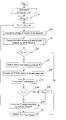
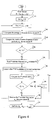
- FIG. 1 is a block diagram illustrating a method of estimating vibration amplitude limits according to an exemplary embodiment.
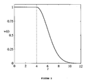
- FIG. 2 is a diagram representing a function for removing old data from a dataset according to an exemplary embodiment.
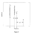
- FIG. 3 is a diagram representing frequency interpolation according to an exemplary embodiment.
- FIG. 4 is a block diagram illustrating a method of detecting outlier data from a dataset according to an exemplary embodiment.
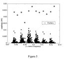
- FIG. 5 is a diagram representing the application of multivariate outlier removal from vibration data according to an exemplary embodiment.
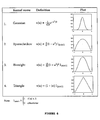
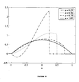
- FIG. 6 is a diagram illustrating a variety of kernel functions according to an exemplary embodiment.
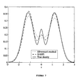
- FIG. 7 is a diagram comparing kernel density estimates obtained using different bandwidth selection methods according to an exemplary embodiment.
- FIG. 8 is a diagram illustrating Epanechnikov boundary kernels for different values according to an exemplary embodiment.
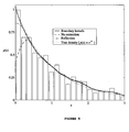
- FIG. 9 is a diagram illustrating the effect of boundary bias on kernel density estimation according to an exemplary embodiment.
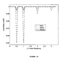
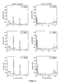
- FIG. 10 is a diagram illustrating the effect of weighting on the alert, alarm, and danger confidence levels with diagnostic frequencies for a chiller according to an exemplary embodiment.
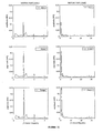
- FIG. 11 is a diagram illustrating amplitude limit envelopes for the motor-vertical position of a chiller according to an exemplary embodiment.
- FIG. 12 is a diagram illustrating amplitude limit envelopes for the compressor-vertical position of a chiller according to an exemplary embodiment.
- the method described in this disclosure uses observed data to identify the probability distribution for the data and then uses the probability distribution to calculate limits for the data. For example, if a user finds that data follows a Gamma probability distribution, then the user can fit the data to a Gamma distribution, and then calculate the limits from the probability distribution. In many instances, vibration data do not follow a single type of distribution, and therefore there is a need to automatically generate the probability distribution from the data itself.
- a preferred embodiment of the invention calculates the probability distribution from the data using the kernel density estimation method, and then uses the estimated probability distribution to calculate the vibration limits.
- Step 1 requires user input while the rest of the steps are executed automatically.
- a vibration analyst specifies the chiller model for which the limits will be calculated as well as the frequency range of the spectrum.
- the frequency range of the spectrum is from F range, low to F range, hi Hz.
- the analyst also specifies the electrical line frequency (e.g., 60 Hz in North America, 50 Hz in Europe) and the importance levels for different frequencies. The importance levels for different frequencies is described in greater detail below.
- a historical database is queried to retrieve all spectra for the specified chiller make and model and the selected frequency range.
- the set “S” denotes the collection of n spectra retrieved from the historical data and the j th member of S is denoted as S j .
- Each spectrum S j consists of frequency and amplitude data.
- the motor frequency for every spectrum S j is calculated by first searching for the highest amplitude in the range 57-60 Hz (60 Hz is the electric line frequency in North America) and then using interpolation or another method to refine the frequency location of the peak.
- an interpolation method may be used such as described by T ECHNICAL A SSOCIATES , C ONCENTRATED V IBRATION S IGNATURE A NALYSIS AND R ELATED C ONDITION M ONITORING T ECHNIQUES (2002).
- FIG. 2 illustrates this method.
- f p may be the frequency value of the highest peak in the range of 57-60 Hz.
- a loop begins for calculating the vibration amplitude limits at different frequencies.
- the limits can be calculated at any frequency, according to a preferred embodiment, the limits are calculated at frequencies spaced less than or equal to N bw /3 to have a good resolution for the amplitude limit spectrum.
- step 6 implements a loop counter, i, from 0 to 2m.
- f i F range , lo + i ⁇ N bw / 3 M _ f ( 4 ) where f i is scaled by the average motor frequency.
- step 8 after the frequency value has been specified at step 7 , vibration data are collected in the frequency range f i ⁇ 2N bw to f i +2N bw from each spectrum S j .
- step 8 involves collecting vibration data in the range f i ⁇ (c ⁇ N bw ), where c is an integer ⁇ 2.
- step 3 had scaled the frequency axis of each spectrum by its motor frequency.
- the data collected in step 8 has two dimensions: frequency and amplitude.
- outlier detection and removal for the two dimensional data collected from step 8 is implemented.
- Outlier removal is helpful to reduce the effect of unusual observations in limits calculation.
- outlier detection procedures are known in the art.
- outlier removal using kernel density estimation may be utilized.
- the sequential Wilk's multivariate outlier detection test may be utilized to determine outliers, as explained by C. C ARONI AND P. P RESCOTR, Sequential Application of Wilk's Multivariate Outlier Test , A PPL . S TATISTICS 41, 355-64 (1992), hereinafter referred to as the “C and P method”.
- the C and P method is well suited to the present embodiment because the data is two-dimensional (frequency and amplitude). The detailed procedure for detecting outliers using the C and P method will now be described.
- the algorithm for detecting multivariate outliers in data is presented in FIG. 4 .
- the procedure presented in FIG. 4 identifies possible outliers in the dataset X.
- the descriptions of the steps of the procedure are presented below.
- the matrix of sums of squares of outer products, A i for the dataset X is computed.
- the i th extreme observation x e,i in the dataset X is found.
- refers to the determinant of the matrix A.
- the i th extreme Wilk's statistic D i is computed.
- the i th critical value i is computed.
- F d, n ⁇ d ⁇ i, (1 ⁇ /(n ⁇ i+1)) is the 100 ⁇ (1 ⁇ /(n ⁇ i+1)) th percentage point for the F distribution with d and (n ⁇ d ⁇ i) degrees of freedom
- ⁇ is the probability of detecting outliers when there are no outliers
- d is the dimensionality of the data.
- a test is performed to determine if the i th critical value D i is less than the critical value ⁇ i (D i ⁇ i ), determined in step 27 .
- extreme observation x e,i is removed from the dataset X. After removing the extreme element x e, i , the number of observations in the dataset X is n ⁇ i. If i equals r, then the process proceeds to step 31 . Otherwise, i is incremented and the process returns to step 21 .
- step 31 the extreme observations that are outliers ⁇ x e,1 , x e,2 , . . . , x e,nout ⁇ are identified.
- the first n out extremes identified at step 25 are considered outliers. However, not all the extreme values determined at step 25 are outliers.
- the C and P method is designed for Gaussian data.
- vibration data does not always follow a Gaussian distribution.
- the C and P method may still be used to process the vibration data because the approach enables the detection of observations that have very high amplitudes compared to a majority of the data.
- the maximum number of expected outliers in the data, r is another parameter of the C and P method.
- a large value for r means that more data points are expected to be outliers, which results in a large computational effort.
- r may be set to be the largest integer less than 0.2 ⁇ n, where n is the number of spectra in the set S to reduce the computational load.
- the vibration database contains data from acceptable as well as faulty machines. Outlier removal is performed to remove the unusual values that are a result of severe faults and/or measurement errors. After outlier removal, the database may still contain data from machines that have large vibration levels, but these data should be included for calculation of amplitude limits in order to observe the full range and distribution of vibration amplitudes.
- the amplitude axis is divided into a fine grid of 1000 points and P(x
- F f i ) is calculated numerically at each of these grid points. This procedure makes calculating the inverse of P(x
- F f i ) at step 11 relatively easy.
- the value x: is calculated such that P(x
- x ⁇ is the 100 ⁇ % confidence limit for the vibration amplitude. Typical values for ⁇ are 0.95, 0.99, etc.
- An exemplary methodology for choosing the value for ⁇ is discussed below.
- the value of x ⁇ can be calculated by a look-up table of P(x
- F f i ) and x grid values from step 10 .
- the process returns back to the beginning of the “For” loop at step 6 and the amplitude limits for a new frequency value are calculated.
- a spectral amplitude limit envelope is obtained at the termination of the “For” loop.
- the vibration analyst can compare the spectrum for a new machine with the calculated limit envelope to determine if any amplitude in the new spectrum violates the limits. If any of the amplitudes violate the limits, then a machine fault is present. In addition, the frequency location of a limit violation provides the vibration analyst with clues about the possible cause of the fault.
- the kernel density estimation method briefly discussed at step 10 above will now be described in greater detail.
- the kernel density method is described in detail by M. P. W AND AND M. C. J ONES , K ERNEL S MOOTHING (1995).
- the kernel density estimation method is also known as the Parzen windows method for density estimation. It attempts to estimate an unknown probability density for a given dataset X.
- Equation (12) There are two known ways of constructing the multivariate density in Equation (12) from univariate kernel functions.
- K s (•) and K P (•) are usually different, the difference between the kernel densities estimated using K S (•) and K p (•) is typically very small.
- the product kernel K P (•) is easier to implement in software, particularly when boundary correction (described below) is not required in all dimensions.
- the product form of the multivariate kernel is used to calculate the density according to a preferred embodiment.
- F and x denote the frequency and the amplitude dimensions, respectively.
- h f and h x are bandwidths of the frequency and amplitude kernels
- f i and x j are the frequency and amplitude values of the j th observation in the dataset, respectively.
- the kernel density estimation method has two important design parameters including the choice of the kernel function and its bandwidth.
- the choice of the kernel function is not particularly important based on the efficiencies of different kernel functions, the choice is useful from a computational perspective for large data sets.
- a Gaussian kernel requires a much larger computational effort than the Epanechnikov kernel.
- a Gaussian boundary kernel requires the numerical calculation of integrals while the expression for the Epanechnikov boundary kernel is obtained analytically.
- the Epanechnikov kernel has the lowest asymptotic mean integrated squared error (AMISE) in estimating the kernel density as well as a low computational cost.
- AMISE asymptotic mean integrated squared error
- the Epanechnikov kernel is the preferred kernel for estimating the probability density.
- the second useful parameter is the kernel bandwidth.
- the kernel bandwidth calculation methods can be divided into two broad categories: (i) first generation rules-of-thumb, and (ii) second generation methods that produce bandwidths close to the optimal value.
- a rule of thumb (ROT) using the sample variance and the inter-quartile-range (IQR) may be used to estimate the bandwidth of the kernels.
- the quantity ⁇ is the sample standard deviation.
- the quantity represents the width estimate based on the inter-quartile range and the factor 1.349 is the inter-quartile-range for a Gaussian distribution with zero mean and unit standard deviation. This expression is valid for univariate data.
- the Sheather-Jones bandwidth selection method may be used to calculate the kernel bandwidth. This method calculates the bandwidth by using a series of “direct-plug-in” equations and is described by S. J. S HEATHER AND M. C. J ONES , A Reliable Data - Based Bandwidth Selection Method for Kernel Density Estimation , J. R OYAL S TATISTICAL S oc . S ER . B, v. 53, 683-90 (1991).
- the Sheather-Jones direct-plug-in (SJ-dpi) method calculates the kernel bandwidth by using fourth and higher order derivatives of the kernel function and requires them to be non-zero and finite. Because the third and higher-order derivatives of the Epanechnikov kernel function presented in this disclosure are zero, the SJ-dpi method cannot be used directly to calculate the bandwidth for the Epanechnikov kernel. To solve this problem, an exemplary method uses a result called the theory of equivalent kernels, which is described by D. W. S COTT , M ULTIVARIATE D ENSITY E STIMATION : T HEORY , V ISUALIZATION AND P RACTICE (1992).
- the bandwidth calculated using one kernel function can easily be transformed to another kernel function.
- the bandwidth is calculated assuming a Gaussian kernel
- the method calculates the bandwidth using the Gaussian kernel and then transforms it for the Epanechnikov kernel using Equation (17).
- h 1 h 2 [ R ⁇ ( ⁇ 1 ) / ⁇ 2 2 ⁇ ( ⁇ 1 ) R ⁇ ( ⁇ 2 ) / ⁇ 2 2 ⁇ ( ⁇ 2 ) ] 1 5 ( 18 ) where ⁇ 2 ( ⁇ ) is the second order moment and R( ⁇ ) is the roughness of the kernel ⁇ .
- ⁇ ⁇ 8 NS 105 32 ⁇ ⁇ ⁇ ⁇ 9 ( 20 ) where n is the sample size.
- ⁇ (6) (0) is the sixth derivative of the kernel function ⁇ evaluated at zero
- ⁇ 2 ( ⁇ ) is the second-order moment for the kernel ⁇ .
- FIG. 7 shows the improvement of the SJ-dpi method over the first generation bandwidth calculation method.
- Kernel density estimates can have large bias near boundaries when the data have lower or upper bounds.
- the vibration amplitudes are always positive, that is, the data have a lower boundary at zero.
- a different set of kernels may be used near the boundary.
- ⁇ L (•) is the boundary kernel
- h and ⁇ x
- v 1 ⁇ ( a ) 3 16 ⁇ ( - a 4 + 2 ⁇ ⁇ a 2 - 1 )
- v 2 ⁇ ( a ) 1 20 ⁇ ( - 3 ⁇ a 5 + 5 ⁇ ⁇ a 3 + 2 ) ( 30 )
- the boundary kernels are used in Equation (13) when ⁇ 1 and the standard kernel is used for ⁇ 1.
- the density estimate using these kernels can also be negative.
- boundary kernels In addition to boundary kernels, two other methods for reducing boundary bias may be utilized such as data reflection and data transformation.
- the data reflection method makes the density estimate “consistent” but still produces estimates with a large boundary bias.
- boundary kernels are needed to reduce the bias at the boundary to the same level as that in the interior.
- the data transformation method is more complicated and computationally intensive than the boundary kernels approach.
- the boundary kernels is a preferred method to reduce the boundary bias in kernel density estimation.
- p ⁇ ( x ) ⁇ e - x if x ⁇ 0 0 if x ⁇ 0.
- the conditional probability density for the amplitude is known, it is used to calculate limits as follows.
- the limits for the vibration amplitudes may be estimated by first numerically integrating the estimated conditional density p(x
- F f) in Equation (14) using Simpson's rule to obtain the cumulative conditional density function P(x
- F f).
- a cutoff value, ⁇ is also specified for the cumulative probability function.
- the amplitude limit x ⁇ is estimated by calculating the inverse of the cumulative probability density function P(x
- F f) at a probability value of ⁇ : P ( x
- diagnostic frequencies There are special frequencies in the vibration spectrum that are called “diagnostic frequencies” because they correspond to the characteristic frequencies of different machine components. Vibration analysts commonly analyze vibrations near these frequencies to detect mechanical faults. Some examples of diagnostic frequencies for chillers are motor, compressor, gear-mesh and blade-pass frequencies.
- a vibration analyst can specify importance levels for different frequencies in the vibration spectrum. For example, for a Chiller A, the motor frequencies are assigned high importance while the blade-pass frequencies and other parts of the spectrum have relatively lower importance levels. The probability cutoffs are determined from the importance level of a frequency.
- a five level importance scheme may be used where each importance level corresponds to a different value for the probability cutoff for each of the alert, alarm and danger limits.
- an importance level of “one” means low importance, while a value of “five” means high importance.
- the probability cutoff values for the five importance levels are presented in Table 1.
- the diagnostic frequencies of a machine e.g., motor, blade-pass, gear-mesh frequencies, etc.
- the default importance level for the entire spectrum except the diagnostic frequencies is set to “one” (low importance).
- Low importance levels typically have high probability cutoff values. These high probability cutoffs result in higher amplitude limits for frequencies that are not very important. Higher amplitude limits for less important frequencies will result in a lower number of false alarms.
- an importance level scheme such as described herein allows the vibration analyst to focus on the important frequencies while retaining the ability to detect faults when unusually high amplitudes are observed at less important frequencies.
- the probability cutoff limits have a sharp discontinuity at the diagnostic frequencies. For example, the importance level changes from “one” to “five” at the motor frequencies and results in an abrupt change in the probability cutoff values. This abrupt change in the probability cutoffs may result in a sharp discontinuity for the amplitude limit envelope at the diagnostic frequencies.
- FIG. 10 shows the probability cutoff levels for the 0-200 Hz spectrum with diagnostic frequencies of half, one, two and three times the motor frequency. The importance levels for these diagnostic frequencies are “five,” “ive,” “four” and “three” respectively.
- vibration spectra for two chillers were obtained and outlier removal and density estimation were performed for every frequency line using methods such as described above.
- the limits were calculated for every frequency line.
- FIGS. 11 and 12 The results for the motor and compressor vertical positions for Chiller A are presented in FIGS. 11 and 12 respectively. These figures show that although it is useful to detect problems at the diagnostic frequencies of motor harmonics, sub-harmonics and blade-pass frequencies, other frequency ranges play a role. For example, a high amplitude of vibration in frequency band 1-1.5 ⁇ motor frequency may signal a bearing fault that will be missed if only the diagnostic frequencies were analyzed.
- the exemplary approach allows the vibration analyst to quickly compare the entire spectrum with the limit envelopes to detect problems in any part of the spectrum.
Abstract
Description
- The present invention relates generally to the field of detecting mechanical faults in HVAC equipment. More specifically, the present invention relates to a methodology for calculating vibration amplitude limits to detect mechanical faults in HVAC equipment such as chillers.
- Timely detection, diagnosis and repair of mechanical problems in machinery such as heating, ventilating and air-conditioning (HVAC) systems is important for efficient operation. Chillers are important components of HVAC systems because they consume a large fraction of energy in a building and require a large capital investment. Severe mechanical faults in chillers typically results in expensive repairs and disruptions to the HVAC system during the repair period. Accordingly, chillers are generally monitored routinely to detect developing mechanical faults.
- A common method for detecting and diagnosing mechanical faults is vibration analysis. By analyzing vibration data from different positions on a chiller, a vibration analyst can detect and diagnose mechanical faults in a machine. Vibration data is commonly available as a spectrum. The vibration analyst can determine a machine's condition by analyzing the vibration amplitude at different frequencies in the spectrum. A vibration analyst typically detects a mechanical fault that requires corrective action when the amplitudes in the vibration spectrum exceed “acceptable” limits. Under many current approaches, the acceptable limits are specified by rules-of-thumb or from a vibration analyst's experience. However, these approaches can be unreliable. For example, limits determined from an individual's experience can be incorrect or inconsistent. Similarly, limits specified by rules-of-thumb are typically generalized to apply to a large number of chillers and are therefore not likely relevant for some particular types of chillers.
- Accordingly, there exists a need for a method of more accurately detecting mechanical faults without having to rely on an individual's knowledge of a system or general rule-of-thumb limits. In particular, it is desirable to be able to derive the limits from historical data using advanced statistical methods. By using statistics and historical data, the estimated limits may be based entirely on the vibration spectrum of each type of chiller. This approach easily allows updating of the amplitude limits when new vibration data from chillers is collected. In addition, because this approach uses statistical methods and not expert knowledge or “rules-of-thumb,” it results in more consistent limits. Many vendors also use rudimentary statistics such as calculating the average and standard deviation of the data to estimate limits. Unfortunately, this approach can result in erroneous limits because vibration data usually don't follow a bell shaped (or Gaussian) probability distribution.
- It would be advantageous to provide a method or the like of a type disclosed in the present application that provides any one or more of these or other advantageous features. The present invention further relates to various features and combinations of features shown and described in the disclosed embodiments. Other ways in which the objects and features of the disclosed embodiments are accomplished will be described in the following specification or will become apparent to those skilled in the art after they have read this specification. Such other ways are deemed to fall within the scope of the disclosed embodiments if they fall within the scope of the claims which follow.
- One embodiment of the present invention relates to a method for determining vibration amplitude limits to detect faults in mechanical equipment. The method comprises estimating a data probability distribution based on data for the mechanical equipment and utilizing the data probability distribution to calculate the vibration amplitude limits.
- Another embodiment of the present invention relates to a method for detecting faults in a chiller based on vibration amplitude limits. The method comprises calculating vibration amplitude limits of the chiller using statistics and historical data for the chiller, estimating an at least two-dimensional density estimate, and weighting the historical data based on when the historical data was generated. The vibration amplitude limits are calculated as a function of frequency for an entire frequency spectrum.
- Another embodiment of the present invention relates to a method for determining vibration amplitude limits of a mechanical device. The method comprises identifying a mechanical device and a frequency range for a spectrum to be analyzed, retrieving vibration spectra comprising individual spectrum for the mechanical device and the frequency range, calculating frequency for the individual spectrum, and identifying the individual spectrum with the smallest number of frequency lines. In addition, the method comprises calculating noise bandwidths and a largest noise bandwidth, removing outlier data, calculating conditional kernel density, and calculating vibration amplitude limits to detect faults in the mechanical device.
-
FIG. 1 is a block diagram illustrating a method of estimating vibration amplitude limits according to an exemplary embodiment. -
FIG. 2 is a diagram representing a function for removing old data from a dataset according to an exemplary embodiment. -
FIG. 3 is a diagram representing frequency interpolation according to an exemplary embodiment. -
FIG. 4 is a block diagram illustrating a method of detecting outlier data from a dataset according to an exemplary embodiment. -
FIG. 5 is a diagram representing the application of multivariate outlier removal from vibration data according to an exemplary embodiment. -
FIG. 6 is a diagram illustrating a variety of kernel functions according to an exemplary embodiment. -
FIG. 7 is a diagram comparing kernel density estimates obtained using different bandwidth selection methods according to an exemplary embodiment. -
FIG. 8 is a diagram illustrating Epanechnikov boundary kernels for different values according to an exemplary embodiment. -
FIG. 9 is a diagram illustrating the effect of boundary bias on kernel density estimation according to an exemplary embodiment. -
FIG. 10 is a diagram illustrating the effect of weighting on the alert, alarm, and danger confidence levels with diagnostic frequencies for a chiller according to an exemplary embodiment. -
FIG. 11 is a diagram illustrating amplitude limit envelopes for the motor-vertical position of a chiller according to an exemplary embodiment. -
FIG. 12 is a diagram illustrating amplitude limit envelopes for the compressor-vertical position of a chiller according to an exemplary embodiment. - Before explaining a number of exemplary embodiments of the invention in detail, it is to be understood that the invention is not limited to the details or methodology set forth in the following description or illustrated in the drawings. The invention is capable of other embodiments or being practiced or carried out in various ways. It is also to be understood that the phraseology and terminology employed herein is for the purpose of description and should not be regarded as limiting.
- In general, the method described in this disclosure uses observed data to identify the probability distribution for the data and then uses the probability distribution to calculate limits for the data. For example, if a user finds that data follows a Gamma probability distribution, then the user can fit the data to a Gamma distribution, and then calculate the limits from the probability distribution. In many instances, vibration data do not follow a single type of distribution, and therefore there is a need to automatically generate the probability distribution from the data itself. A preferred embodiment of the invention calculates the probability distribution from the data using the kernel density estimation method, and then uses the estimated probability distribution to calculate the vibration limits.
- An exemplary methodology for calculating vibration limits from historical data will now be discussed. This methodology is shown in
FIG. 1 .Step 1 requires user input while the rest of the steps are executed automatically. - At
step 1, a vibration analyst specifies the chiller model for which the limits will be calculated as well as the frequency range of the spectrum. The frequency range of the spectrum is from Frange, low to Frange, hi Hz. The analyst also specifies the electrical line frequency (e.g., 60 Hz in North America, 50 Hz in Europe) and the importance levels for different frequencies. The importance levels for different frequencies is described in greater detail below. - At
step 2, a historical database is queried to retrieve all spectra for the specified chiller make and model and the selected frequency range. The set “S” denotes the collection of n spectra retrieved from the historical data and the jth member of S is denoted as Sj. Each spectrum Sj consists of frequency and amplitude data. - At
step 3, a motor frequency Mf, j(j=1, . . . , n) is estimated for every spectrum Sj and the frequency axis of Sj is scaled by its motor frequency, Mf, j . Scaling the frequency axis by the motor frequency reduces the variation in the spectra due to differences in motor speeds. The motor frequency for every spectrum Sj is calculated by first searching for the highest amplitude in the range 57-60 Hz (60 Hz is the electric line frequency in North America) and then using interpolation or another method to refine the frequency location of the peak. For example, an interpolation method may be used such as described by TECHNICAL ASSOCIATES , CONCENTRATED VIBRATION SIGNATURE ANALYSIS AND RELATED CONDITION MONITORING TECHNIQUES (2002).FIG. 2 illustrates this method. According to an exemplary embodiment illustrated inFIG. 3 , while locating the motor frequency from the vibration spectrum, fp may be the frequency value of the highest peak in the range of 57-60 Hz. If Ap is the amplitude at fp, fs and As are the frequency and amplitude of the line having an amplitude closest to Ap, and Δf is the spacing between adjacent frequency lines, then the interpolated frequency fi may be calculated as: - At
step 4, the spectrum having the smallest number of frequency lines in S is found. If the number of frequency lines in spectrum Sj is mj, then
The value of m results in the calculation of the largest noise bandwidth Nbw in S. - At
step 5, the largest noise bandwidth Nbw in S is calculated as:
where {overscore (M)}f is the average value of the machine frequency for n spectra:
According to an exemplary embodiment, the factor 1.5 is utilized assuming that a Hanning window was used for calculation of the spectrum from its time waveform. - At
step 6, a loop begins for calculating the vibration amplitude limits at different frequencies. Although the limits can be calculated at any frequency, according to a preferred embodiment, the limits are calculated at frequencies spaced less than or equal to Nbw/3 to have a good resolution for the amplitude limit spectrum. Using results fromstep 4, there are 2m+1 frequency values where the limits are calculated. Thus,step 6 implements a loop counter, i, from 0 to 2m. - At
step 7, a frequency value at which the amplitude limits will be estimated is calculated:
where fi is scaled by the average motor frequency. - At
step 8, after the frequency value has been specified atstep 7, vibration data are collected in the frequency range fi−2Nbw to fi+2Nbw from each spectrum Sj. In general,step 8 involves collecting vibration data in the range fi±(c×Nbw), where c is an integer ≧2. The preferred value c=2 ensures that all data within the noise bandwidth is included in the density calculation and the computational load is at a minimum. A value of c<2 would result in elimination of data just outside the noise bandwidth. Recall thatstep 3 had scaled the frequency axis of each spectrum by its motor frequency. The data collected instep 8 has two dimensions: frequency and amplitude. - At
step 9, outlier detection and removal for the two dimensional data collected fromstep 8 is implemented. Outlier removal is helpful to reduce the effect of unusual observations in limits calculation. Outliers are observations that appear to be inconsistent with the majority of data in a dataset. These observations are preferably removed from the data because they may corrupt the data analysis and can produce misleading results. For example, the average for the dataset, X={10, 9, 11, 8, 12, 50, 11, 30, 8}, is 16.6, even though the majority of the data are centered around 10. Theobservations 30 and 50 push the average to a higher value that suggests that most of the observations are centered around 16, which could be a misleading result. These observations also appear to be much larger than the majority of the data, and thus are called outliers. The average becomes 9.86 when these extreme observations are removed from the dataset, a result that is consistent with the majority of observations. - Many types of outlier detection procedures are known in the art. According to an exemplary embodiment, outlier removal using kernel density estimation may be utilized. According to a preferred embodiment, the sequential Wilk's multivariate outlier detection test may be utilized to determine outliers, as explained by C. C
ARONI AND P. PRESCOTR, Sequential Application of Wilk's Multivariate Outlier Test, APPL . STATISTICS 41, 355-64 (1992), hereinafter referred to as the “C and P method”. The C and P method is well suited to the present embodiment because the data is two-dimensional (frequency and amplitude). The detailed procedure for detecting outliers using the C and P method will now be described. - The algorithm for detecting multivariate outliers in data is presented in
FIG. 4 . Given a dataset X={x1, x2, . . . , xn}, with n observations in d dimensions, and an estimate of the upper bound r for the number of outliers, the procedure presented inFIG. 4 identifies possible outliers in the dataset X. The descriptions of the steps of the procedure are presented below. Atstep 21, the number of outliers is initialized to zero by setting nout=0. Atstep 22, the average {overscore (x)} of the observations for dataset X is computed as:
where xj is a member of the dataset X and n equals the number of observations in X. - At
step 23, the matrix of sums of squares of outer products, Ai, for the dataset X is computed. The matrix sum of squares is determined as: - At
step 24, a test is performed to determine whether the matrix sum of squares is zero (Ai=0). If this matrix is zero, then all of the observations in dataset X have the same value and there are no outliers in the remaining observations in dataset X. To prevent division by the determinant of a zero matrix at step 25, the process moves to step 31 when the matrix sum of squares instep 24 equals zero. Otherwise, the process advances to step 25. - At step 25, the ith extreme observation xe,i in the dataset X is found. The most extreme observation xe,i can be identified where its removal results in the smallest value of Wi=|Ai|/|Ai−1|, where Ai−1 is the matrix obtained by removing the most extreme observation in the previous step. The notation |A| refers to the determinant of the matrix A.
- At
step 26, the ith extreme Wilk's statistic Di is computed. The Wilk's statistic is determined as: - At
step 27, the ith critical value i is computed. The C and P method utilizes the following relation for determining the critical value:
where Fd, n−d−i, (1−α/(n−i+1)) is the 100×(1−α/(n−i+1))th percentage point for the F distribution with d and (n−d−i) degrees of freedom, α is the probability of detecting outliers when there are no outliers, and d is the dimensionality of the data. - At
step 28, a test is performed to determine if the ith critical value Di is less than the critical value γi(Di<γi), determined instep 27. Atstep 29, the number of outliers nout is set equal to i (nout=i). Atstep 30, extreme observation xe,i is removed from the dataset X. After removing the extreme element xe, i, the number of observations in the dataset X is n−i. If i equals r, then the process proceeds to step 31. Otherwise, i is incremented and the process returns to step 21. Atstep 31, the extreme observations that are outliers {xe,1, xe,2, . . . , xe,nout} are identified. The first nout extremes identified at step 25 are considered outliers. However, not all the extreme values determined at step 25 are outliers. - The C and P method is designed for Gaussian data. However, vibration data does not always follow a Gaussian distribution. Despite this limitation, the C and P method may still be used to process the vibration data because the approach enables the detection of observations that have very high amplitudes compared to a majority of the data.
- The maximum number of expected outliers in the data, r, is another parameter of the C and P method. A large value for r means that more data points are expected to be outliers, which results in a large computational effort. According to an exemplary embodiment, r may be set to be the largest integer less than 0.2×n, where n is the number of spectra in the set S to reduce the computational load.
- The vibration database contains data from acceptable as well as faulty machines. Outlier removal is performed to remove the unusual values that are a result of severe faults and/or measurement errors. After outlier removal, the database may still contain data from machines that have large vibration levels, but these data should be included for calculation of amplitude limits in order to observe the full range and distribution of vibration amplitudes. The application of the C and P method is presented in
FIG. 5 for sample data from a chiller at f=0.5. - Referring back to
FIG. 1 , atstep 10, the conditional kernel density p(x|F=fi) is calculated, where x is the amplitude and F represents the frequency axis. An exemplary procedure for calculating p(x|F=fi) from the two dimensional data is discussed below. Atstep 10, the cumulative probability function, P(x|F=fi), is also calculated by numerically integrating the density p(x|F=fi) from zero to x:
The amplitude axis is divided into a fine grid of 1000 points and P(x|F=fi) is calculated numerically at each of these grid points. This procedure makes calculating the inverse of P(x|F=fi) atstep 11 relatively easy. - At
step 11, the value x: is calculated such that P(x|F=fi)=β, where β is a specified probability cutoff. Thus, xβ is the 100×β % confidence limit for the vibration amplitude. Typical values for β are 0.95, 0.99, etc. An exemplary methodology for choosing the value for β is discussed below. The value of xβ can be calculated by a look-up table of P(x|F=fi) and x grid values fromstep 10. After the completion ofstep 11, the process returns back to the beginning of the “For” loop atstep 6 and the amplitude limits for a new frequency value are calculated. A spectral amplitude limit envelope is obtained at the termination of the “For” loop. The vibration analyst can compare the spectrum for a new machine with the calculated limit envelope to determine if any amplitude in the new spectrum violates the limits. If any of the amplitudes violate the limits, then a machine fault is present. In addition, the frequency location of a limit violation provides the vibration analyst with clues about the possible cause of the fault. - The kernel density estimation method briefly discussed at
step 10 above will now be described in greater detail. The kernel density method is described in detail by M. P. WAND AND M. C. JONES , KERNEL SMOOTHING (1995). The kernel density estimation method is also known as the Parzen windows method for density estimation. It attempts to estimate an unknown probability density for a given dataset X. The probability density estimate at a point x for a one-dimensional dataset with n data points is given by:
where, xj is the jth observation of the dataset X, h is called the bandwidth that characterizes the spread of the kernel, and κ(•) is a kernel density function that is symmetric and satisfies the condition:
Some common univariate kernel density functions, κ(•), are listed inFIG. 6 . Thenotation 1{|u|≦1} means: - To calculate the kernel density for two-dimensional vibration data (e.g., frequency and amplitude directions), an expression should be utilized for the kernel density estimation in two or more dimensions. In general, Equation (9) is extended to d dimensions by replacing the univariate kernel κ(u) by a d-dimensional kernel K (u), and the bandwidth h by a bandwidth matrix H. Then, the d-dimensional kernel density estimate is written as:
where |•| denotes the matrix determinant. There are two known ways of constructing the multivariate density in Equation (12) from univariate kernel functions. One option is to use a spherically symmetric multivariate kernel KS(u)=cκ,dκ((utu)1/2), where cκ,d is a constant dependent on the univariate kernel κ(•), and the dimensionality. A second option is to use a multivariate product kernel
Although Ks(•) and KP(•) are usually different, the difference between the kernel densities estimated using KS(•) and Kp(•) is typically very small. The product kernel KP(•) is easier to implement in software, particularly when boundary correction (described below) is not required in all dimensions. Thus, the product form of the multivariate kernel is used to calculate the density according to a preferred embodiment. - For the two-dimensional vibration data, F and x denote the frequency and the amplitude dimensions, respectively. Then, the expression for the kernel density using the product kernel in these two dimensions is written as:
In Equation (13), hf and hx are bandwidths of the frequency and amplitude kernels, and fi and xj are the frequency and amplitude values of the jth observation in the dataset, respectively. - To calculate the vibration amplitude limits at a given frequency value F=f, the conditional probability density p(x|F=fi) is first calculated from the joint probability density p(x, F). Conditional density is then used to calculate the limits. The conditional probability density of the vibration amplitude (x) for a given frequency value (F=f) is calculated as:
- The kernel density estimation method has two important design parameters including the choice of the kernel function and its bandwidth. First, although the choice of the kernel function is not particularly important based on the efficiencies of different kernel functions, the choice is useful from a computational perspective for large data sets. For example, a Gaussian kernel requires a much larger computational effort than the Epanechnikov kernel. Also, a Gaussian boundary kernel requires the numerical calculation of integrals while the expression for the Epanechnikov boundary kernel is obtained analytically.
- The Epanechnikov kernel has the lowest asymptotic mean integrated squared error (AMISE) in estimating the kernel density as well as a low computational cost. Thus, the Epanechnikov kernel is the preferred kernel for estimating the probability density.
- The second useful parameter is the kernel bandwidth. The kernel bandwidth calculation methods can be divided into two broad categories: (i) first generation rules-of-thumb, and (ii) second generation methods that produce bandwidths close to the optimal value.
- A rule of thumb (ROT) using the sample variance and the inter-quartile-range (IQR) may be used to estimate the bandwidth of the kernels. According to an exemplary embodiment, a robust estimate of the kernel width, h, is,
h=0.9×λ×n −1/5 (15)
where,
The quantity σ is the sample standard deviation. The inter-quartile-range (IQR) is computed as the difference between the 75th percentile (Q3) and the 25th percentile (Q1) of the data. Thus, IQR=Q3−Q1. The quantity represents the width estimate based on the inter-quartile range and the factor 1.349 is the inter-quartile-range for a Gaussian distribution with zero mean and unit standard deviation. This expression is valid for univariate data. - Second generation methods are designed to produce bandwidths that are close to the optimum but require a larger computational effort. According to an exemplary embodiment, the Sheather-Jones bandwidth selection method may be used to calculate the kernel bandwidth. This method calculates the bandwidth by using a series of “direct-plug-in” equations and is described by S. J. S
HEATHER AND M. C. JONES , A Reliable Data-Based Bandwidth Selection Method for Kernel Density Estimation, J. ROYAL STATISTICAL Soc . SER . B, v. 53, 683-90 (1991). - The Sheather-Jones direct-plug-in (SJ-dpi) method calculates the kernel bandwidth by using fourth and higher order derivatives of the kernel function and requires them to be non-zero and finite. Because the third and higher-order derivatives of the Epanechnikov kernel function presented in this disclosure are zero, the SJ-dpi method cannot be used directly to calculate the bandwidth for the Epanechnikov kernel. To solve this problem, an exemplary method uses a result called the theory of equivalent kernels, which is described by D. W. S
COTT , MULTIVARIATE DENSITY ESTIMATION : THEORY , VISUALIZATION AND PRACTICE (1992). By using this theory, the bandwidth calculated using one kernel function can easily be transformed to another kernel function. For example, if the bandwidth is calculated assuming a Gaussian kernel, then the equivalent bandwidth for the Epanechnikov kernel is:
h Epanech=2.214×h Gaussian (17)
Because the Gaussian kernel function has infinite number of non-zero and finite derivatives, the method calculates the bandwidth using the Gaussian kernel and then transforms it for the Epanechnikov kernel using Equation (17). The bandwidths h1 and h2 of two kernels κ1 and κ2 are related as:
where μ2(κ) is the second order moment and R(κ) is the roughness of the kernel κ. - The Sheather-Jones direct-plug-in method assuming a Gaussian kernel is described as follows. First, calculate the estimate of scale (λ) for the data. It is preferred to use the smaller of the sample standard deviation (σ) and the normalized interquartile range (IQR) as a scale estimate:
- Second, calculate the normal-scale approximation,
where n is the sample size. Third, calculate the first approximation of the bandwidth:
where κ(6)(0) is the sixth derivative of the kernel function κ evaluated at zero, and μ2(κ) is the second-order moment for the kernel κ. Here κ=Gaussian kernel is assumed. Fourth, calculate the second approximation of the bandwidth using the fourth derivative of the kernel and the kernel estimator {circumflex over (ψ)}6(g1): - Finally, calculate the bandwidth using the kernel roughness function R(κ) and the kernel estimator {circumflex over (ψ)}4(g2):
- A comparison of the kernel density estimates using the first generation method and Sheather-Jones direct-plug-in bandwidths is presented in
FIG. 7 for a multi-modal density
The kernel density estimate using the first generation bandwidth method completely misses the middle peak at x=0, while the density estimate using the SJ-dpi bandwidth is able to reveal the tri-modal structure of the data. Thus,FIG. 7 shows the improvement of the SJ-dpi method over the first generation bandwidth calculation method. - The difference between the actual density and the calculated kernel density is called the bias of the kernel density. Kernel density estimates can have large bias near boundaries when the data have lower or upper bounds. For the present embodiment on chiller vibration data, the vibration amplitudes are always positive, that is, the data have a lower boundary at zero. To correct the error in estimating density near the lower boundary (near zero), a different set of kernels may be used near the boundary. For kernels with a [−1, 1] support, such as the Epanechnikov kernel, boundary kernels may be calculated as:
where κL(•) is the boundary kernel, κ(•) is a kernel function defined in Table 1 with a [−1, 1] support, u=(x−xi)|h and α=x|h. The coefficients v1(≢)(l=0, 1, 2) are defined as:
For the Epanechnikov kernel, the coefficients vl(α) are:
The boundary kernels are used in Equation (13) when α<1 and the standard kernel is used for α≧1. The Epanechnikov boundary kernels for different values of the parameter α=x/h are presented inFIG. 8 . - Because the boundary kernels have negative values, the density estimate using these kernels can also be negative. Thus, in order to obtain a positive density estimate, the negative density may be truncated to zero and then the density estimate may be re-scaled as:
such that p(x) now satisfies p(x)≧0 and - In addition to boundary kernels, two other methods for reducing boundary bias may be utilized such as data reflection and data transformation. The data reflection method makes the density estimate “consistent” but still produces estimates with a large boundary bias. Thus, boundary kernels are needed to reduce the bias at the boundary to the same level as that in the interior. The data transformation method is more complicated and computationally intensive than the boundary kernels approach. Thus, the boundary kernels is a preferred method to reduce the boundary bias in kernel density estimation.
- A simple example illustrating the effect of boundary bias on kernel density estimation is presented in
FIG. 9 for the exponential density p(x)=e−x. The exponential density has a lower boundary at x=0 so that:
In this example, one thousand observations were sampled from the exponential distribution and the data were used to estimate the kernel density.FIG. 9 shows that with no boundary bias correction, the kernel density estimate near the boundary is very different from the true density. The estimate is better with the reflection method, while the boundary kernels approach produces very accurate results. - Once the conditional probability density for the amplitude is known, it is used to calculate limits as follows. The limits for the vibration amplitudes may be estimated by first numerically integrating the estimated conditional density p(x|F=f) in Equation (14) using Simpson's rule to obtain the cumulative conditional density function P(x|F=f). A cutoff value, β, is also specified for the cumulative probability function. Then, the amplitude limit xβ is estimated by calculating the inverse of the cumulative probability density function P(x|F=f) at a probability value of β:
P(x|F=f)=β (26) - Typically, a vibration analyst sets three levels of amplitude limits that are referred to as the “alert,” “alarm” and “danger” limits. Common values for the probability cutoffs for these limits are β=0.95, 0.99 and 0.995 respectively.
TABLE 1 Probability cutoff limits for different importance levels. Importance β Level Alert Alarm Danger 1 (low) 0.9995 0.9999 0.99995 2 0.999 0.9995 0.9999 3 0.995 0.999 0.9995 4 0.99 0.995 0.999 5 (high) 0.95 0.99 0.995 - There are special frequencies in the vibration spectrum that are called “diagnostic frequencies” because they correspond to the characteristic frequencies of different machine components. Vibration analysts commonly analyze vibrations near these frequencies to detect mechanical faults. Some examples of diagnostic frequencies for chillers are motor, compressor, gear-mesh and blade-pass frequencies.
- In the exemplary methodology, a vibration analyst can specify importance levels for different frequencies in the vibration spectrum. For example, for a Chiller A, the motor frequencies are assigned high importance while the blade-pass frequencies and other parts of the spectrum have relatively lower importance levels. The probability cutoffs are determined from the importance level of a frequency.
- A five level importance scheme may be used where each importance level corresponds to a different value for the probability cutoff for each of the alert, alarm and danger limits. According to an exemplary embodiment, an importance level of “one” means low importance, while a value of “five” means high importance. The probability cutoff values for the five importance levels are presented in Table 1. Typically, the diagnostic frequencies of a machine (e.g., motor, blade-pass, gear-mesh frequencies, etc.) have high importance levels, while other parts of the spectrum have lower importance. Hence, the default importance level for the entire spectrum except the diagnostic frequencies is set to “one” (low importance).
- Low importance levels typically have high probability cutoff values. These high probability cutoffs result in higher amplitude limits for frequencies that are not very important. Higher amplitude limits for less important frequencies will result in a lower number of false alarms. Thus, an importance level scheme such as described herein allows the vibration analyst to focus on the important frequencies while retaining the ability to detect faults when unusually high amplitudes are observed at less important frequencies.
- Examination of the foregoing importance level scheme reveals that the probability cutoff limits have a sharp discontinuity at the diagnostic frequencies. For example, the importance level changes from “one” to “five” at the motor frequencies and results in an abrupt change in the probability cutoff values. This abrupt change in the probability cutoffs may result in a sharp discontinuity for the amplitude limit envelope at the diagnostic frequencies. To have a continuous transition between the cutoff limits, a weighting scheme is used to smooth the probability cutoff values near the diagnostic frequencies:
- In Equation (34), βf is the probability cutoff value for frequency F=f, βdef is the default probability cutoff corresponding to the lowest importance level, and βdiag is the probability cutoff limit for the closest diagnostic frequency fdiag. If the frequency f is between two diagnostic frequencies that are closer than 12×Nbw from each other, then linear interpolation may be used to determine the probability cutoff value between the two diagnostic frequencies, otherwise Equation (34) is used. This situation occurs while calculating the probability cutoff values between 2×motor and electrical frequencies.
FIG. 10 shows the probability cutoff levels for the 0-200 Hz spectrum with diagnostic frequencies of half, one, two and three times the motor frequency. The importance levels for these diagnostic frequencies are “five,” “ive,” “four” and “three” respectively. - According to an exemplary embodiment, vibration spectra for two chillers (Chiller A and B) were obtained and outlier removal and density estimation were performed for every frequency line using methods such as described above. In addition, the limits were calculated for every frequency line.
- The results for the motor and compressor vertical positions for Chiller A are presented in
FIGS. 11 and 12 respectively. These figures show that although it is useful to detect problems at the diagnostic frequencies of motor harmonics, sub-harmonics and blade-pass frequencies, other frequency ranges play a role. For example, a high amplitude of vibration in frequency band 1-1.5×motor frequency may signal a bearing fault that will be missed if only the diagnostic frequencies were analyzed. The exemplary approach allows the vibration analyst to quickly compare the entire spectrum with the limit envelopes to detect problems in any part of the spectrum. - It is important to note that the above-described preferred embodiments are illustrative only. Although the invention has been described in conjunction with specific embodiments thereof, those skilled in the art will appreciate that numerous modifications are possible without materially departing from the novel teachings and advantages of the subject matter described herein. Accordingly, these and all other such modifications are intended to be included within the scope of the present invention as defined in the appended claims. The order or sequence of any process or method steps may be varied or re-sequenced according to alternative embodiments. In the claims, any means-plus-function clause is intended to cover the structures described herein as performing the recited function and not only structural equivalents but also equivalent structures. Other substitutions, modifications, changes and omissions may be made in the design, operating conditions and arrangements of the preferred and other exemplary embodiments without departing from the spirit of the present invention.
Claims (36)
Priority Applications (1)
| Application Number | Priority Date | Filing Date | Title |
|---|---|---|---|
| US10/805,807 US7124637B2 (en) | 2004-03-22 | 2004-03-22 | Determining amplitude limits for vibration spectra |
Applications Claiming Priority (1)
| Application Number | Priority Date | Filing Date | Title |
|---|---|---|---|
| US10/805,807 US7124637B2 (en) | 2004-03-22 | 2004-03-22 | Determining amplitude limits for vibration spectra |
Publications (2)
| Publication Number | Publication Date |
|---|---|
| US20050204818A1 true US20050204818A1 (en) | 2005-09-22 |
| US7124637B2 US7124637B2 (en) | 2006-10-24 |
Family
ID=34984743
Family Applications (1)
| Application Number | Title | Priority Date | Filing Date |
|---|---|---|---|
| US10/805,807 Expired - Lifetime US7124637B2 (en) | 2004-03-22 | 2004-03-22 | Determining amplitude limits for vibration spectra |
Country Status (1)
| Country | Link |
|---|---|
| US (1) | US7124637B2 (en) |
Cited By (13)
| Publication number | Priority date | Publication date | Assignee | Title |
|---|---|---|---|---|
| US20070185686A1 (en) * | 2006-02-06 | 2007-08-09 | Johnson Controls Technology Company | State-based method and apparatus for evaluating the performance of a control system |
| US20080183424A1 (en) * | 2007-01-25 | 2008-07-31 | Johnson Controls Technology Company | Method and system for assessing performance of control systems |
| US20080277486A1 (en) * | 2007-05-09 | 2008-11-13 | Johnson Controls Technology Company | HVAC control system and method |
| US20090065596A1 (en) * | 2007-05-09 | 2009-03-12 | Johnson Controls Technology Company | Systems and methods for increasing building space comfort using wireless devices |
| US20110151815A1 (en) * | 2009-12-17 | 2011-06-23 | Electronics And Telecommunications Research Institute | System and method for identifying gaussian radio noise |
| US20110190909A1 (en) * | 2010-02-01 | 2011-08-04 | Johnson Controls Technology Company | Systems and methods for increasing feedback controller response times |
| GB2481782A (en) * | 2010-06-21 | 2012-01-11 | Optimized Systems And Solutions Ltd | Asset health monitoring |
| KR101293906B1 (en) | 2009-12-17 | 2013-08-06 | 한국전자통신연구원 | System and method for discrimination of gaussian radio noise |
| US20150204757A1 (en) * | 2014-01-17 | 2015-07-23 | United States Of America As Represented By The Secretary Of The Navy | Method for Implementing Rolling Element Bearing Damage Diagnosis |
| US9992355B2 (en) | 2016-02-02 | 2018-06-05 | Fuji Xerox Co., Ltd. | Diagnostic apparatus, diagnostic system, and non-transitory computer readable medium |
| CN109426656A (en) * | 2017-08-28 | 2019-03-05 | 株洲中车时代电气股份有限公司 | A kind of shock response spectrum test profile formulating method |
| US11287156B2 (en) * | 2019-03-11 | 2022-03-29 | Qingdao Haier Air-Conditioning Electronic Co., Ltd | Method for controlling air conditioner compressor frequency based on vibration of pipeline |
| US20230014054A1 (en) * | 2021-07-13 | 2023-01-19 | GM Global Technology Operations LLC | System for audibly detecting precursors of material fracture for a specimen under test |
Families Citing this family (36)
| Publication number | Priority date | Publication date | Assignee | Title |
|---|---|---|---|---|
| DE102005040192A1 (en) * | 2005-08-25 | 2007-03-01 | Robert Bosch Gmbh | Method and device for detecting squeaking noises |
| US7827813B2 (en) * | 2007-01-30 | 2010-11-09 | Johnson Controls Technology Company | Adaptive real-time optimization control |
| US20080179408A1 (en) * | 2007-01-30 | 2008-07-31 | Johnson Controls Technology Company | Sensor-free optimal control of air-side economizer |
| WO2009012269A2 (en) * | 2007-07-17 | 2009-01-22 | Johnson Controls Technology Company | Extremum seeking control with actuator saturation control |
| WO2009012282A2 (en) | 2007-07-17 | 2009-01-22 | Johnson Controls Technology Company | Extremum seeking control with reset control |
| US20090067363A1 (en) * | 2007-07-31 | 2009-03-12 | Johnson Controls Technology Company | System and method for communicating information from wireless sources to locations within a building |
| DE102008021360A1 (en) * | 2008-04-29 | 2009-11-05 | Siemens Aktiengesellschaft | Method and device for detecting bearing damage |
| US7866213B2 (en) * | 2008-06-18 | 2011-01-11 | Siemens Energy, Inc. | Method of analyzing non-synchronous vibrations using a dispersed array multi-probe machine |
| GB0902730D0 (en) * | 2009-02-18 | 2009-04-01 | Oxford Biosignals Ltd | Method and apparatus for monitoring and analyzing vibrations in rotary machines |
| US8239168B2 (en) * | 2009-06-18 | 2012-08-07 | Johnson Controls Technology Company | Systems and methods for fault detection of air handling units |
| US8788097B2 (en) | 2009-06-22 | 2014-07-22 | Johnson Controls Technology Company | Systems and methods for using rule-based fault detection in a building management system |
| US9753455B2 (en) | 2009-06-22 | 2017-09-05 | Johnson Controls Technology Company | Building management system with fault analysis |
| US9286582B2 (en) | 2009-06-22 | 2016-03-15 | Johnson Controls Technology Company | Systems and methods for detecting changes in energy usage in a building |
| US8532839B2 (en) | 2009-06-22 | 2013-09-10 | Johnson Controls Technology Company | Systems and methods for statistical control and fault detection in a building management system |
| US8600556B2 (en) | 2009-06-22 | 2013-12-03 | Johnson Controls Technology Company | Smart building manager |
| US9196009B2 (en) | 2009-06-22 | 2015-11-24 | Johnson Controls Technology Company | Systems and methods for detecting changes in energy usage in a building |
| US8731724B2 (en) | 2009-06-22 | 2014-05-20 | Johnson Controls Technology Company | Automated fault detection and diagnostics in a building management system |
| US9606520B2 (en) | 2009-06-22 | 2017-03-28 | Johnson Controls Technology Company | Automated fault detection and diagnostics in a building management system |
| US11269303B2 (en) | 2009-06-22 | 2022-03-08 | Johnson Controls Technology Company | Systems and methods for detecting changes in energy usage in a building |
| US10739741B2 (en) | 2009-06-22 | 2020-08-11 | Johnson Controls Technology Company | Systems and methods for detecting changes in energy usage in a building |
| US8781608B2 (en) * | 2009-07-31 | 2014-07-15 | Johnson Controls Technology Company | Systems and methods for improved start-up in feedback controllers |
| WO2011100255A2 (en) | 2010-02-09 | 2011-08-18 | Johnson Controls Technology Company | Systems and methods for measuring and verifying energy savings in buildings |
| US8473080B2 (en) | 2010-05-10 | 2013-06-25 | Johnson Controls Technology Company | Control of cooling towers for chilled fluid systems |
| US8412357B2 (en) | 2010-05-10 | 2013-04-02 | Johnson Controls Technology Company | Process control systems and methods having learning features |
| US9429092B2 (en) | 2010-07-16 | 2016-08-30 | Cummins Inc. | Fault detection and response techniques |
| US9390388B2 (en) | 2012-05-31 | 2016-07-12 | Johnson Controls Technology Company | Systems and methods for measuring and verifying energy usage in a building |
| US11639881B1 (en) | 2014-11-19 | 2023-05-02 | Carlos A. Rosero | Integrated, continuous diagnosis, and fault detection of hydrodynamic bearings by capacitance sensing |
| US9778639B2 (en) | 2014-12-22 | 2017-10-03 | Johnson Controls Technology Company | Systems and methods for adaptively updating equipment models |
| US10684030B2 (en) | 2015-03-05 | 2020-06-16 | Honeywell International Inc. | Wireless actuator service |
| US9953474B2 (en) | 2016-09-02 | 2018-04-24 | Honeywell International Inc. | Multi-level security mechanism for accessing a panel |
| US11016003B2 (en) | 2016-11-17 | 2021-05-25 | Ez Pulley Llc | Systems and methods for detection and analysis of faulty components in a rotating pulley system |
| CN106971027B (en) * | 2017-03-09 | 2020-06-23 | 西安建筑科技大学 | Water chilling unit fault feature selection method based on DR-BN model |
| CN106951671B (en) * | 2017-05-25 | 2020-03-24 | 中国石油大学(华东) | Oil-submersible electric pump assembly quality grade classification method based on vibration information |
| US10311703B1 (en) | 2018-02-09 | 2019-06-04 | Computational Systems, Inc. | Detection of spikes and faults in vibration trend data |
| US10832509B1 (en) | 2019-05-24 | 2020-11-10 | Ademco Inc. | Systems and methods of a doorbell device initiating a state change of an access control device and/or a control panel responsive to two-factor authentication |
| US10789800B1 (en) | 2019-05-24 | 2020-09-29 | Ademco Inc. | Systems and methods for authorizing transmission of commands and signals to an access control device or a control panel device |
Citations (16)
| Publication number | Priority date | Publication date | Assignee | Title |
|---|---|---|---|---|
| US4931949A (en) * | 1988-03-21 | 1990-06-05 | Monitoring Technology Corporation | Method and apparatus for detecting gear defects |
| US5086775A (en) * | 1990-11-02 | 1992-02-11 | University Of Rochester | Method and apparatus for using Doppler modulation parameters for estimation of vibration amplitude |
| US5922963A (en) * | 1997-06-13 | 1999-07-13 | Csi Technology, Inc. | Determining narrowband envelope alarm limit based on machine vibration spectra |
| US6138045A (en) * | 1998-08-07 | 2000-10-24 | Arch Development Corporation | Method and system for the segmentation and classification of lesions |
| US6208944B1 (en) * | 1997-06-26 | 2001-03-27 | Pruftechnik Dieter Busch Ag | Method for determining and displaying spectra for vibration signals |
| US6301572B1 (en) * | 1998-12-02 | 2001-10-09 | Lockheed Martin Corporation | Neural network based analysis system for vibration analysis and condition monitoring |
| US6314204B1 (en) * | 1998-11-03 | 2001-11-06 | Compaq Computer Corporation | Multiple mode probability density estimation with application to multiple hypothesis tracking |
| US6370957B1 (en) * | 1999-12-31 | 2002-04-16 | Square D Company | Vibration analysis for predictive maintenance of rotating machines |
| US6438981B1 (en) * | 2000-06-06 | 2002-08-27 | Jay Daniel Whiteside | System for analyzing and comparing current and prospective refrigeration packages |
| US6629058B2 (en) * | 2000-04-20 | 2003-09-30 | Rion Co., Ltd. | Fault diagnosis method and apparatus |
| US6651012B1 (en) * | 2001-05-24 | 2003-11-18 | Simmonds Precision Products, Inc. | Method and apparatus for trending and predicting the health of a component |
| US6697759B2 (en) * | 2000-03-20 | 2004-02-24 | Abb Research Ltd. | Method of determining speed of rotation of a motor and a computer software product to carry out the method |
| US6792360B2 (en) * | 2001-12-04 | 2004-09-14 | Skf Condition Monitoring, Inc. | Harmonic activity locator |
| US6816810B2 (en) * | 2000-03-23 | 2004-11-09 | Invensys Systems, Inc. | Process monitoring and control using self-validating sensors |
| US20050021212A1 (en) * | 2003-07-24 | 2005-01-27 | Gayme Dennice F. | Fault detection system and method using augmented data and fuzzy logic |
| US6980910B1 (en) * | 2001-03-20 | 2005-12-27 | Johnson Controls Technology Company | Extensions to dynamically configurable process for diagnosing faults in rotating machines |
-
2004
- 2004-03-22 US US10/805,807 patent/US7124637B2/en not_active Expired - Lifetime
Patent Citations (17)
| Publication number | Priority date | Publication date | Assignee | Title |
|---|---|---|---|---|
| US4931949A (en) * | 1988-03-21 | 1990-06-05 | Monitoring Technology Corporation | Method and apparatus for detecting gear defects |
| US5086775A (en) * | 1990-11-02 | 1992-02-11 | University Of Rochester | Method and apparatus for using Doppler modulation parameters for estimation of vibration amplitude |
| US5922963A (en) * | 1997-06-13 | 1999-07-13 | Csi Technology, Inc. | Determining narrowband envelope alarm limit based on machine vibration spectra |
| US6208944B1 (en) * | 1997-06-26 | 2001-03-27 | Pruftechnik Dieter Busch Ag | Method for determining and displaying spectra for vibration signals |
| US6138045A (en) * | 1998-08-07 | 2000-10-24 | Arch Development Corporation | Method and system for the segmentation and classification of lesions |
| US6314204B1 (en) * | 1998-11-03 | 2001-11-06 | Compaq Computer Corporation | Multiple mode probability density estimation with application to multiple hypothesis tracking |
| US6301572B1 (en) * | 1998-12-02 | 2001-10-09 | Lockheed Martin Corporation | Neural network based analysis system for vibration analysis and condition monitoring |
| US6370957B1 (en) * | 1999-12-31 | 2002-04-16 | Square D Company | Vibration analysis for predictive maintenance of rotating machines |
| US6697759B2 (en) * | 2000-03-20 | 2004-02-24 | Abb Research Ltd. | Method of determining speed of rotation of a motor and a computer software product to carry out the method |
| US6816810B2 (en) * | 2000-03-23 | 2004-11-09 | Invensys Systems, Inc. | Process monitoring and control using self-validating sensors |
| US6629058B2 (en) * | 2000-04-20 | 2003-09-30 | Rion Co., Ltd. | Fault diagnosis method and apparatus |
| US6662584B1 (en) * | 2000-06-06 | 2003-12-16 | Jay Daniel Whiteside | System for analyzing and comparing current and prospective refrigeration packages |
| US6438981B1 (en) * | 2000-06-06 | 2002-08-27 | Jay Daniel Whiteside | System for analyzing and comparing current and prospective refrigeration packages |
| US6980910B1 (en) * | 2001-03-20 | 2005-12-27 | Johnson Controls Technology Company | Extensions to dynamically configurable process for diagnosing faults in rotating machines |
| US6651012B1 (en) * | 2001-05-24 | 2003-11-18 | Simmonds Precision Products, Inc. | Method and apparatus for trending and predicting the health of a component |
| US6792360B2 (en) * | 2001-12-04 | 2004-09-14 | Skf Condition Monitoring, Inc. | Harmonic activity locator |
| US20050021212A1 (en) * | 2003-07-24 | 2005-01-27 | Gayme Dennice F. | Fault detection system and method using augmented data and fuzzy logic |
Cited By (18)
| Publication number | Priority date | Publication date | Assignee | Title |
|---|---|---|---|---|
| US7289936B2 (en) | 2006-02-06 | 2007-10-30 | Johnson Controls Technology Company | State-based method and apparatus for evaluating the performance of a control system |
| US20070185686A1 (en) * | 2006-02-06 | 2007-08-09 | Johnson Controls Technology Company | State-based method and apparatus for evaluating the performance of a control system |
| US20080183424A1 (en) * | 2007-01-25 | 2008-07-31 | Johnson Controls Technology Company | Method and system for assessing performance of control systems |
| US7496472B2 (en) * | 2007-01-25 | 2009-02-24 | Johnson Controls Technology Company | Method and system for assessing performance of control systems |
| US20080277486A1 (en) * | 2007-05-09 | 2008-11-13 | Johnson Controls Technology Company | HVAC control system and method |
| US20090065596A1 (en) * | 2007-05-09 | 2009-03-12 | Johnson Controls Technology Company | Systems and methods for increasing building space comfort using wireless devices |
| KR101293906B1 (en) | 2009-12-17 | 2013-08-06 | 한국전자통신연구원 | System and method for discrimination of gaussian radio noise |
| US20110151815A1 (en) * | 2009-12-17 | 2011-06-23 | Electronics And Telecommunications Research Institute | System and method for identifying gaussian radio noise |
| US20110190909A1 (en) * | 2010-02-01 | 2011-08-04 | Johnson Controls Technology Company | Systems and methods for increasing feedback controller response times |
| US8428755B2 (en) | 2010-02-01 | 2013-04-23 | Johnson Controls Technology Company | Systems and methods for increasing feedback controller response times |
| GB2481782A (en) * | 2010-06-21 | 2012-01-11 | Optimized Systems And Solutions Ltd | Asset health monitoring |
| US20150204757A1 (en) * | 2014-01-17 | 2015-07-23 | United States Of America As Represented By The Secretary Of The Navy | Method for Implementing Rolling Element Bearing Damage Diagnosis |
| US9992355B2 (en) | 2016-02-02 | 2018-06-05 | Fuji Xerox Co., Ltd. | Diagnostic apparatus, diagnostic system, and non-transitory computer readable medium |
| AU2016210766B2 (en) * | 2016-02-02 | 2018-07-05 | Fujifilm Business Innovation Corp. | Diagnostic apparatus, diagnostic system, and program |
| CN109426656A (en) * | 2017-08-28 | 2019-03-05 | 株洲中车时代电气股份有限公司 | A kind of shock response spectrum test profile formulating method |
| US11287156B2 (en) * | 2019-03-11 | 2022-03-29 | Qingdao Haier Air-Conditioning Electronic Co., Ltd | Method for controlling air conditioner compressor frequency based on vibration of pipeline |
| US20230014054A1 (en) * | 2021-07-13 | 2023-01-19 | GM Global Technology Operations LLC | System for audibly detecting precursors of material fracture for a specimen under test |
| US11624730B2 (en) * | 2021-07-13 | 2023-04-11 | GM Global Technology Operations LLC | System for audibly detecting precursors of material fracture for a specimen under test |
Also Published As
| Publication number | Publication date |
|---|---|
| US7124637B2 (en) | 2006-10-24 |
Similar Documents
| Publication | Publication Date | Title |
|---|---|---|
| US7124637B2 (en) | Determining amplitude limits for vibration spectra | |
| US6957172B2 (en) | Complex signal decomposition and modeling | |
| US11644391B2 (en) | Fault diagnosis method under convergence trend of center frequency | |
| US7321845B2 (en) | Method and system for removing very low frequency noise from a time-based data set | |
| US7865334B2 (en) | Method of and apparatus for evaluating the performance of a control system | |
| US6804628B2 (en) | System for surveillance of spectral signals | |
| US20150219530A1 (en) | Systems and methods for event detection and diagnosis | |
| US7769561B2 (en) | Robust sensor correlation analysis for machine condition monitoring | |
| Yashchin | Monitoring variance components | |
| US20130158901A1 (en) | Method and System for Detecting Unbalance in Power Grids | |
| US20150006972A1 (en) | Method for Detecting Anomalies in a Time Series Data with Trajectory and Stochastic Components | |
| US7949497B2 (en) | Machine condition monitoring using discontinuity detection | |
| US8494036B2 (en) | Resource adaptive spectrum estimation of streaming data | |
| US20030028349A1 (en) | System for monitoring non-coincident, nonstationary process signals | |
| JP2009110262A (en) | Filter device, filtering method for filter device and filtering program | |
| CN112697483A (en) | LMD multi-scale fluctuation analysis state monitoring method and device | |
| US6281814B1 (en) | Data conversion method, data converter, and program storage medium | |
| US20030035376A1 (en) | Derivation of composite step-function response | |
| Baruah et al. | An autonomous diagnostics and prognostics framework for condition-based maintenance | |
| ÜSTÜNDAĞ et al. | Estimating parameters of sinusoids from noisy data using Bayesian inference with simulated annealing | |
| Lopez et al. | Unsupervised fault detection using semidefinite programming | |
| Schmidt | Development of Effective Gearbox Fault Diagnosis Methodologies Utilising Various Levels of Prior Knowledge | |
| Wiig et al. | Trend-based transmission system diagnosis | |
| Schmidt | A cost-effective diagnostic methodology using probabilistic approaches for gearboxes operating under non-stationary conditions | |
| CN115541231A (en) | Rotating machinery state monitoring method based on impact component probability distribution measurement |
Legal Events
| Date | Code | Title | Description |
|---|---|---|---|
| AS | Assignment |
Owner name: JOHNSON CONTROLS TECHNOLOGY COMPANY, MICHIGAN Free format text: ASSIGNMENT OF ASSIGNORS INTEREST;ASSIGNORS:SHINGHAL, ASHISH;SEEM, JOHN E.;MUENCH, MARK J.;REEL/FRAME:015131/0093 Effective date: 20040319 |
|
| STCF | Information on status: patent grant |
Free format text: PATENTED CASE |
|
| FPAY | Fee payment |
Year of fee payment: 4 |
|
| FPAY | Fee payment |
Year of fee payment: 8 |
|
| MAFP | Maintenance fee payment |
Free format text: PAYMENT OF MAINTENANCE FEE, 12TH YEAR, LARGE ENTITY (ORIGINAL EVENT CODE: M1553) Year of fee payment: 12 |
|
| AS | Assignment |
Owner name: JOHNSON CONTROLS TYCO IP HOLDINGS LLP, WISCONSIN Free format text: NUNC PRO TUNC ASSIGNMENT;ASSIGNOR:JOHNSON CONTROLS TECHNOLOGY COMPANY;REEL/FRAME:058959/0764 Effective date: 20210806 |
|
| AS | Assignment |
Owner name: TYCO FIRE & SECURITY GMBH, SWITZERLAND Free format text: ASSIGNMENT OF ASSIGNORS INTEREST;ASSIGNOR:JOHNSON CONTROLS TYCO IP HOLDINGS LLP;REEL/FRAME:066800/0629 Effective date: 20240201 |