US20040109561A1 - Lean multiplication of multi-precision numbers over GF(2m) - Google Patents
Lean multiplication of multi-precision numbers over GF(2m) Download PDFInfo
- Publication number
- US20040109561A1 US20040109561A1 US10/636,326 US63632603A US2004109561A1 US 20040109561 A1 US20040109561 A1 US 20040109561A1 US 63632603 A US63632603 A US 63632603A US 2004109561 A1 US2004109561 A1 US 2004109561A1
- Authority
- US
- United States
- Prior art keywords
- polynomial
- word
- subproducts
- multiplication
- algorithm
- Prior art date
- Legal status (The legal status is an assumption and is not a legal conclusion. Google has not performed a legal analysis and makes no representation as to the accuracy of the status listed.)
- Granted
Links
Images


Classifications
-
- H—ELECTRICITY
- H04—ELECTRIC COMMUNICATION TECHNIQUE
- H04L—TRANSMISSION OF DIGITAL INFORMATION, e.g. TELEGRAPHIC COMMUNICATION
- H04L9/00—Cryptographic mechanisms or cryptographic arrangements for secret or secure communications; Network security protocols
- H04L9/30—Public key, i.e. encryption algorithm being computationally infeasible to invert or user's encryption keys not requiring secrecy
- H04L9/3093—Public key, i.e. encryption algorithm being computationally infeasible to invert or user's encryption keys not requiring secrecy involving Lattices or polynomial equations, e.g. NTRU scheme
-
- G—PHYSICS
- G06—COMPUTING; CALCULATING OR COUNTING
- G06F—ELECTRIC DIGITAL DATA PROCESSING
- G06F7/00—Methods or arrangements for processing data by operating upon the order or content of the data handled
- G06F7/60—Methods or arrangements for performing computations using a digital non-denominational number representation, i.e. number representation without radix; Computing devices using combinations of denominational and non-denominational quantity representations, e.g. using difunction pulse trains, STEELE computers, phase computers
- G06F7/72—Methods or arrangements for performing computations using a digital non-denominational number representation, i.e. number representation without radix; Computing devices using combinations of denominational and non-denominational quantity representations, e.g. using difunction pulse trains, STEELE computers, phase computers using residue arithmetic
- G06F7/724—Finite field arithmetic
- G06F7/725—Finite field arithmetic over elliptic curves
-
- H—ELECTRICITY
- H04—ELECTRIC COMMUNICATION TECHNIQUE
- H04L—TRANSMISSION OF DIGITAL INFORMATION, e.g. TELEGRAPHIC COMMUNICATION
- H04L9/00—Cryptographic mechanisms or cryptographic arrangements for secret or secure communications; Network security protocols
- H04L9/32—Cryptographic mechanisms or cryptographic arrangements for secret or secure communications; Network security protocols including means for verifying the identity or authority of a user of the system or for message authentication, e.g. authorization, entity authentication, data integrity or data verification, non-repudiation, key authentication or verification of credentials
- H04L9/3247—Cryptographic mechanisms or cryptographic arrangements for secret or secure communications; Network security protocols including means for verifying the identity or authority of a user of the system or for message authentication, e.g. authorization, entity authentication, data integrity or data verification, non-repudiation, key authentication or verification of credentials involving digital signatures
- H04L9/3252—Cryptographic mechanisms or cryptographic arrangements for secret or secure communications; Network security protocols including means for verifying the identity or authority of a user of the system or for message authentication, e.g. authorization, entity authentication, data integrity or data verification, non-repudiation, key authentication or verification of credentials involving digital signatures using DSA or related signature schemes, e.g. elliptic based signatures, ElGamal or Schnorr schemes
-
- G—PHYSICS
- G06—COMPUTING; CALCULATING OR COUNTING
- G06F—ELECTRIC DIGITAL DATA PROCESSING
- G06F2207/00—Indexing scheme relating to methods or arrangements for processing data by operating upon the order or content of the data handled
- G06F2207/72—Indexing scheme relating to groups G06F7/72 - G06F7/729
- G06F2207/7209—Calculation via subfield, i.e. the subfield being GF(q) with q a prime power, e.g. GF ((2**m)**n) via GF(2**m)
Definitions
- This application relates to the efficient multiplication of large numbers in a variety of different environments, including cryptography.
- Multi-precision numbers In the field of digital circuits, for instance, the binary representation of a large number can be stored in multiple words, wherein each word has a fixed length of n bits depending on the word size supported by the associated hardware or software.
- adding and subtracting multi-precision numbers can be performed relatively efficiently, multi-precision multiplication is much more complex and creates a significant bottleneck in applications using multi-precision arithmetic.
- One area that is affected by the complexity of multi-precision multiplication is cryptography.
- Many cryptographic algorithms including the Diffie-Hellman key exchange algorithm, elliptic curve cryptography, and the Elliptic Curve Digital Signature Algorithm (ECDSA), involve the multi-precision multiplication of very large numbers.
- elliptic curve systems perform multi-precision arithmetic on 128- to 256-bit numbers, while systems based on exponentiation may employ 1024- to 2048-bit numbers.
- Another technique involves embedding GF(2 m ) in a larger ring R p where the arithmetic operations can be performed efficiently. See J. H. Silverman, Fast Multiplication in Finite Field GF (2 N ), Cryptographic Hardware and Embedded Systems, pp. 122-134 (1999). This method, however, works only when m+1 is a prime, and 2 is a primitive root modulo m+1.
- Another technique involves using a standard basis with coefficients in a subfield GF(2 r ). See E. De Win et al., A Fast Software Implementation for Arithmetic Operations in GF(2 n ), Advances in Cryptology—ASIACRYPT 96, pp. 65-76 (1996); J.
- Methods and apparatus for multiplying multi-precision numbers over GF(2 m ) using a polynomial representation are disclosed.
- the disclosed methods may be used in a number of different applications that utilize multi-precision arithmetic.
- the method can be used to generate various cryptographic parameters.
- a private key and a base point are multiplied using one of the disclosed methods to obtain a product that is associated with a public key.
- the private key and the base point are multi-precision polynomials.
- the disclosed methods may similarly be used in a signature generation or signature verification process (e.g., the Elliptic Curve Digital Signature Algorithm (ECDSA)).
- EDSA Elliptic Curve Digital Signature Algorithm
- a method in an exemplary embodiment, includes representing the first polynomial and the second polynomial as an array of n words, wherein n is an integer.
- a recursive algorithm is used to decompose a multiplication of the first polynomial and the second polynomial into a weighted sum of iteratively smaller subproducts.
- a nonrecursive algorithm is used to complete the multiplication when a size of the smaller subproducts is less than or equal to a predetermined size, the predetermined size being at least two words.
- the recursive multiplication algorithm may be, for instance, a Karatsuba-Ofman algorithm, and the predetermined size may be, for example, six words.
- the nonrecursive multiplication algorithm may be optimized so that it operates more efficiently.
- the nonrecursive algorithm may exclude pairs of redundant subproducts, or store and reuse previously calculated intermediate values.
- the previously calculated intermediate values may be part of a weighted sum of subproducts having special weights.
- a method of nonrecursively multiplying a first polynomial and a second polynomial over GF(2) is disclosed.
- a first polynomial and a second polynomial are represented as n words, where n is an integer greater than one.
- the partial result is updated by adding any remaining one-word subproducts.
- the method may also include identifying and excluding pairs of redundant one-word subproducts.
- intermediate calculations may be stored in a memory and reused.
- a method of deriving an algorithm for multiplying a first polynomial and a second polynomial over GF(2) is disclosed.
- the product of a first polynomial and a second polynomial is decomposed into a weighted sum of one-word subproducts. Pairs of redundant one-word subproducts are identified and removed from the weighted sum, resulting in a revised weighted sum having fewer XOR operations.
- the first or second polynomial is padded with zeros so that the polynomial has an even number of words. In this implementation, the zero-padded polynomials may be excluded from the revised weighted sum.
- These one-word subproducts can be calculated in a weighted sum by a process of storing and reusing the intermediate calculations.
- the disclosed methods may be implemented in a variety of different software and hardware environments. Any of the disclosed methods may be implemented, for example, as a set of computer-executable instructions stored on a computer-readable medium.
- FIG. 1 is a flowchart showing a general method of multiplying multi-precision polynomials over GF(2 m ).
- FIG. 2 is a block diagram of an exemplary recursion tree having two levels of recursion.
- FIG. 3 is a block diagram of an exemplary recursion tree having three levels of recursion.
- FIG. 4 is a block diagram showing a selected path on the recursion tree of FIG. 3.
- FIG. 5 is a flowchart showing a general method of nonrecursively multiplying multi-precision polynomials over GF(2 m ).
- FIG. 6 is a first block diagram illustrating the operation of the method of FIGS. 1 and 5 using the recursion tree of FIG. 2.
- FIG. 7 is a second block diagram illustrating the operation of the method of FIGS. 1 and 5 using the recursion tree of FIG. 2.
- FIG. 8 is a third block diagram illustrating the operation of the method of FIGS. 1 and 5 using the recursion tree of FIG. 2.
- FIG. 9 is a block diagram of a general-purpose computer configured to perform multi-precision multiplication according to the disclosed methods.
- FIG. 10 is a block diagram of a cryptographic system configured to perform multi-precision multiplication according to the disclosed methods and to output a cryptographic parameter.
- the disclosed methods can be implemented in a variety of different environments, including a general-purpose computer, an application-specific computer or in various other environments known in the art.
- environments including a general-purpose computer, an application-specific computer or in various other environments known in the art.
- the elements in GF(2 m ) can be represented in various bases.
- the standard basis representation for GF(2 m ) is used.
- the operations on these elements are performed modulo a fixed irreducible polynomial of degree m.
- standard basis multiplication in GF(2 m ) has two phases.
- the first phase consists of multiplying two polynomials over GF(2 m ) and the second phase consists of reducing the result modulo an irreducible polynomial of degree m.
- the complexity of standard polynomial multiplication is O(m 2 ). Modulo reduction can be an even more time-consuming operation because it involves division.
- both phases of standard basis multiplication in GF(2 m ) are quite costly.
- the cost of the first phase can be decreased by using the Karatsuba-Ofman Algorithm (KOA) to multiply the polynomials over GF(2 m ).
- the KOA is a multiplication algorithm whose asymptotic complexity is O(m 1.58 ).
- the second phase can also be decreased by choosing an irreducible polynomial with a small number of terms. In particular, a trinomial or pentanomial can be used as the irreducible polynomial.
- a trinomial is a polynomial 1+x a +x m with only three terms
- a pentanomial is a polynomial 1+x a +x b +x c +x m with only five terms.
- the complexity of the modulo reduction operation with a trinomial or a pentanomial is O(m). Further, a trinomial or a pentanomial can be found for any field size m ⁇ 1000.
- the coefficients of the polynomials over GF(2 m ) are 0 or 1 and operations on these coefficients are performed according to modulo two arithmetic.
- addition and subtraction of the coefficients is equivalent to performing XOR operations.
- the addition and subtraction of two polynomials can be performed by XORing the corresponding coefficients.
- polynomial multiplication also depends on the XOR addition/subtraction operation because polynomial multiplication involves a series of coefficient additions.
- polynomials For purposes of this disclosure, bold face variables denote polynomials. Although these polynomials are functions of x, the x argument is omitted for the sake of presentation. Thus, a polynomial denoted by a(x) in the traditional notation will be denoted by a.
- a nw ⁇ 1 0) by zero padding.
- the polynomial a[i] be defined from the coefficients in the ith word as follows:
- the coefficients of the polynomial a are stored in n words.
- a polynomial a over GF(2 m ) can be viewed as an n-word array.
- the polynomial a[k #l] can be viewed as a subarray of a.
- k and l are the index and length parameters.
- the value of k points to the first word of the subarray and shows the position of this word in a, while l gives the length of the subarray in words.
- MULGF2 multiplies two one-word polynomials, writes the lower word of the result into S, and writes the higher word into C.
- no general-purpose processor contains an instruction to perform the MULGF2 operation.
- MULGF2(a[i],b[j]) can be emulated as follows:
- MULGF2 consists of a sequence of shifts and XOR operations because the polynomial multiplication involves a sequence of shifts and additions. In the operation outlined above, for instance, the addition is the bitwise XOR operation.
- the Karatsuba-Ofman algorithm is a divide-and-conquer technique used to perform large multiplications.
- large multiplication may involve the multiplication of multiplicands comprised of a large number of words.
- the KOA computes a large multiplication using the results of the smaller multiplications.
- the KOA computes these smaller multiplications using the results of still smaller multiplications. This process continues recursively until the multiplication becomes relatively small (e.g., until the multiplicands are reduced to one word) such that they may be computed directly without any recursion.
- the KOA algorithm may be modified such that the recursions are stopped early and a bottom-level multiplication is performed using some nonrecursive algorithms.
- These nonrecursive algorithms may be derived from the KOA by removing its recursions.
- the algorithms may be optimized by exploiting the arithmetic of the polynomials over GF(2 m ). Consequently, the complexity and recursion overhead can be reduced.
- this modified embodiment of the KOA is termed the LKOA, or “lean” implementation of the KOA.
- n ⁇ n 2 ⁇ + ⁇ n 2 ⁇ ,
- n is an integer.
- the operand a may be split into a ⁇ n/2 ⁇ -word polynomial a L and a ⁇ n 2 ⁇ ,
- a L and a H are two half-sized polynomials defined from the first ⁇ n 2 ⁇
- a L contains the coefficients of the lower-order terms of a
- a H contains the coefficients of the higher-order terms.
- Equation (13) The general concept of the KOA is to express a multiplication in terms of three half-sized multiplications, as in Equation (13). Consequently, one multiplication operation can be saved at the expense of performing more additions. Because the complexity of multiplication is quadratic, while the complexity of addition is linear, this substitution is advantageous for large values of n.
- the KOA computes a product from three half-sized products. In this same fashion, the KOA computes each of the half-sized products from three quarter-sized products. This process continues recursively until the products get very small (e.g., until the multiplicands are reduced to one word) and can be computed quickly using classical methods.
- the following exemplary recursive function implements the KOA for the polynomials over GF(2 m ).
- Step 1 n is evaluated. If n is one (i.e., if the inputs are one-word inputs), the inputs are multiplied using classical methods and the result returned. Otherwise, the function continues to the remaining steps.
- Steps 2 through 5 two pairs of half-sized polynomials (a L , b L ) and (a H , b H ) are generated from the lower- and higher-order words of the inputs.
- Steps 6 and 7 another pair, (a M , b M ), is obtained by adding a L with b L and a H with b H .
- Steps 8, 9, and 10 these three pairs are multiplied. These multiplications are performed by three recursive calls to the KOA function and yield the subproducts low, mid, and high.
- Step 1 of the KOA function (as outlined above) can be modified.
- the recursion can be stopped when n ⁇ n 0 where n 0 is some predetermined integer.
- a nonrecursive function can then be called to perform the remaining multiplication.
- a variety of different nonrecursive algorithms can be used to multiply the polynomials of size n ⁇ n 0 .
- the polynomials are multiplied on a word-by-word basis, as shown above in the section discussing polynomial multiplication over GF(2 m ).
- a series of nonrecursive algorithms derived from the KOA can be used. These algorithms are each specific to a fixed input size and multiply 2, 3, . . . n-word polynomials respectively.
- the algorithms may be used in a variety of different combinations and subcombinations with one another. For instance, one particular embodiment uses the 2, 3, 4, 5, and 6-word nonrecursive multiplication algorithms described below in combination with the KOA.
- the details of the particular algorithms described may be modified in a number of ways (e.g., the sequence in which the various subproducts are computed may be altered) without departing from the scope of the present disclosure.
- KOA2, KOA3, KOA4, KOA5 and KOA6 are the algorithms derived from the KOA. To obtain these algorithms, the recursions of the KOA, as well as the inherent redundancies in the KOA, are removed by exploiting the arithmetic of the polynomials over GF(2 m ). As noted above, this type of implementation is termed a lean implementation of the KOA, or LKOA.
- FIG. 1 is a flowchart 100 showing a general method of implementing the LKOA.
- two n-word operands a and b are obtained or received.
- the operands a and b comprise multiple words of one or more bits and represent a polynomial in GF(2 m ).
- a recursive algorithm is used to decompose the multiplication of a and b into a weighted sum of smaller subproducts.
- the recursive algorithm utilized may be the KOA or a similar divide-and-conquer algorithm.
- the decomposition continues until the size of the operands of the subproducts reaches a predetermined size.
- the recursive algorithm is used to decompose the products until the operands are six words or less.
- process block 116 shows that a nonrecursive algorithm is used to determine the smaller subproducts.
- the nonrecursive algorithm used may, for instance, be one of the nonrecursive algorithms described below, or another nonrecursive algorithm that efficiently determines the relevant subproduct.
- the values of these subproducts are used in the weighted sum of process block 112 to complete the calculation.
- the final value of the weighted sum is returned.
- two operands in GF(2 m ) can be multiplied together in two phases.
- the polynomial multiplication in the first phase may be performed on a word-by-word basis using the straightforward MULGF2 multiplication algorithm described above. According to this method, however, the first phase is quadratic in time (i.e., O(m 2 )).
- the LKOA may be used to perform the first phase of polynomial multiplication. Because the LKOA runs in less than quadratic time, even for small values of m, the overall time for multiplication is decreased. The LKOA runs faster than the straightforward multiplication algorithm because it trades multiplications in favor of additions. In particular, the LKOA reduces the number of 1-word multiplications (MULGF2) at the expense of more 1-word additions (XOR).
- the LKOA can be used to multiply polynomials with no or little recursion.
- the nonrecursive function KOA6 is called for the computation.
- the LKOA multiplies 16-word polynomials only two levels of recursive calls are used. In the first recursion level, the input size is reduced to 8-word polynomials. In the second recursion level, the input size is reduced to 4-word polynomials, and the inputs are multiplied by the nonrecursive function KOA4.
- the result of the polynomial multiplication is reduced with a trinomial or pentanomial of degree m.
- This computation has a linear time of O(m).
- the implementation of the reduction with a trinomial or pentanomial, for example, is relatively simple and straightforward. See, e.g., R. Schroeppel et al., Fast Key Exchange with Elliptic Curve Systems , Advances in Cryptology—CRYPTO 95, pp. 43-56 (1995).
- a recursion tree is a diagram that depicts the recursions in an algorithm. Recursion trees can be particularly helpful in the analysis of recursive algorithms like the KOA that may call themselves more than once in a recursion step.
- the recursion tree of an algorithm can be thought of as a hierarchical tree structure wherein each branch represents a recursive call of the algorithm.
- FIG. 2 shows an exemplary recursion tree 200 that depicts the multiplication of two exemplary polynomials using an algorithm similar to the KOA.
- the recursion stops when the subproducts reach a size of one word, at which point they can be calculated using classical methods.
- the polynomials 1+x+x 3 +x 4 and 1+x 3 +x 5 are multiplied together.
- FIG. 1+x+x 3 +x 4 and 1+x 3 +x 5 are multiplied together.
- these polynomials are written as a string of two-bit words (i.e., as three words) showing the binary value of each polynomial's coefficients.
- the first polynomial 1+x+x 3 +x 4 is denoted as “110110”
- the second polynomial 1+x 3 +x 5 is denoted as “100101.”
- the initial call to the algorithm is represented by the root 210 of the tree 200 .
- the recursive calls made by the initial call constitute the first level of recursion 220 and are represented by the first-level branches 222 , 224 , 226 emerging from the root 210 .
- the recursive calls made by these recursive calls constitute the second level of recursion 230 and are represented in the recursion tree 200 by the second-level branches 231 through 236 emerging from the first-level branches 222 , 224 .
- branch 226 does not have any second-level branches stemming from it because branch 226 represents the product of one-word operands and can be calculated using classical methods (e.g., a MULGF 2 operation supporting 2 -bit words).
- a branch emerging from another branch may be called a “child.”
- the branch from which the child stems may be called the “parent.”
- branch 231 is the child of branch 222 .
- a branch represents a particular recursive call
- its children represents the recursive calls made by that call.
- a “caller-callee” relationship in an algorithm corresponds to a “parent-child” relationship in the recursion tree. If a recursive call made at some recursion level doesn't make any recursive call at the next level, the branch representing it in the tree has no further children, and may be called a “leaf.”
- branches 222 and 224 In the recursion tree depicted in FIG. 2, two recursive calls are made by the branches 222 and 224 . Thus, three branches, representing a recursive KOA function, emerge from each of these branches.
- the leaves 231 through 236 and 226 represent the multiplication of one-word inputs, which do not make any recursive calls because they can be calculated using classical methods. Generally speaking, the size of the input parameters are reduced by half in each successive recursion level in the recursion tree. Thus, it is known that at some level, the branches will have one-word inputs and cease to make any further recursive calls.
- Recursive tree terminology may be used to describe the KOA or a similar divide-and-conquer algorithm. For example, if one recursive call invokes another, the first recursive call may be referred to as the parent, and the latter recursive call as the child. Thus, a branch may be used as a synonym for a recursive call, and a leaf as a synonym for a recursive call with one-word inputs. Additionally, a path is defined as a sequence of branches from the root in which each branch is a child of the previous one.
- branch 222 in FIG. 2 This branch is a call to the KOA function described above. It has two inputs, “1101” and “1001”. From these inputs, the branch 222 generates the half-sized pairs (a L , b L ), (a M , b M ) and (a H , b H ) (or (11,10), (10,11), and (01,01), respectively). Its children take these pairs as inputs, multiply them, and return the subproducts low, mid, and high. Then, at Step 11, the subproducts are combined in a weighted sum to obtain the value of the product of “1101” and “1001.”
- a branch either takes the input pair (a L , b L ) from its parent and returns the subproduct low, takes the input pair (a H , b H ) and returns the subproduct high, or takes the input pair (a M , b M ) and returns the subproduct mid.
- these first, second, and third types of branches are called low, high, and mid branches respectively. This classification of the branches is given in Table 1 below.
- a branch have the n-word inputs a and b, and the output t.
- Equation (14) It can be seen from Equation (14) how the product t is decomposed into the subproducts weighted by the polynomials in z.
- the sizes of these subproducts can be determined from the variable declarations in the KOA function. Table 2 below gives the sizes and the weights of each subproduct in terms of n. Note that the subproducts are computed by the children and the decomposed product t is computed by the parent. As noted above, n is the input size of this parent branch and the decomposed product t is comprised of 2n words.
- RootProduct the product computed by the root
- leaf-products the products computed by the leaves
- the product RootProduct can be expressed in terms of the leaf-products.
- the products computed by the branches on the paths between the root and the leaves can be recursively decomposed TABLE 2
- the input sizes and weights of subproducts computed by children branches computed subproduct size weight Low Child low 2 ⁇ ⁇ n 2 ⁇ 1 + z ⁇ n 2 ⁇ Mid Child mid 2 ⁇ ⁇ n 2 ⁇ z ⁇ n 2 ⁇ High Child high 2 ⁇ ⁇ n 2 ⁇ z ⁇ n 2 ⁇ + z 2 ⁇ ⁇ n 2 ⁇
- RootProduct ⁇ ⁇ ⁇ i ⁇ LeafProduct i ⁇ Weight i ( 15 )
- LeafProduct i is a particular leaf-product
- Weight i is a polynomial in z.
- FIG. 3 shows a recursion tree 300 illustrating the multiplication of 9-word polynomials a and b.
- the polynomials are reduced to smaller subproducts (i.e., a′,a′′,a′′′) until the individual subproducts have one-word operands, shown in FIG. 3 at the third recursion level.
- FIG. 4 illustrates this path on the recursion tree 300 .
- path 400 originates at the root 410 (i.e., t), and proceeds to its mid child 412 (t′), then to its high grandchild 414 (t′′), and finally to its low grandgrandchild 416 (t′′′).
- the recursive decomposition of the products t, t′, and t′′ is illustrated in Table 3.
- n is the input size of the branch computing the decomposed product, and the decomposed product is comprised of 2n words.
- t′ and two other subproducts emerge. In Table 3, only t′ is shown. The other subproducts are omitted for the sake of presentation.
- Equation (15) can be useful only if the values of LeafProduct i are also known.
- the leaves compute LeafProduct i 's by multiplying their 1-word inputs.
- LeafA and LeafB denote the inputs of the leaf computing LeafProduct i for some i. Then,
- LeafProduct i LeafA LeafB (16)
- LeafProduct i the inputs LeafA and LeafB must be found.
- the inputs of the leaves and the branches are defined from the inputs of their parent in Steps 2 through 7 of the KOA function. Note that all these inputs are actually derived from the inputs of the root, which is the ancestor of the all the branches and the leaves.
- RootA and RootB denote the inputs of the root. Also, let a and b denote the inputs of an arbitrary branch. Then, a and b are in the following form:
- a and b are the appropriate subarrays of the root's inputs or the sum of such subarrays. This is because Steps 2 through 7 of the KOA function, where the inputs of the children are generated from the inputs of the parent, involves only two basic operations: (1) partitioning into subarrays; (2) and adding subarrays. Note that in Equation (17), the subarrays which define a and the subarrays which define b have the same the indices and lengths. This results from the fact that the first and second inputs of a branch are generated in the same way, except that the first input is generated from the words of RootA, while the second input is generated from the words of RootB.
- LeafA and LeafB have the following form:
- the leaf-products can be determined as the products of these inputs.
- the inputs of a branch are generated from the inputs of its parent.
- the inputs of the root's children must first be determined from the inputs of the root. Then, the process can be recursively continued until the inputs of the leaves are obtained.
- Table 4 which is referred to in Proposition 1 and provided below, gives the indices and lengths describing the children's inputs in terms of those describing the parent's input. Table 4 can be used recursively to obtain the indices and lengths describing the inputs of the branches from the higher hierarchy to the lower. Eventually, the indices and lengths describing the inputs of the leaves can be found. Then, the inputs of the leaves can be obtained by adding the subarrays identified by these indices and lengths.
- n is the size of the inputs a and b.
- the size of a and b is the length of the longest subarray in Equation (17).
- n max(l 1 ,l 2 , . . . ,l r ) (20)
- Equation (19) can be more particularly explained as follows:
- a L and b L are the lower halves of a and b (i.e., the first ⁇ n 2 ⁇
- the subarrays defining a L and b L are the lower parts of those defining a and b.
- the lower part of a subarray is its first ⁇ n 2 ⁇
- a H and b H are the higher halves of a and b (i.e., the remaining parts of a and b after their first ⁇ n 2 ⁇
- the subarrays defining a H and b H are the higher parts of those defining a and b.
- the higher part of a subarray is its words from the ⁇ n 2 ⁇
- a M (b M ) is the sum of the a L and a H (b L and b H ).
- the inputs are given in the first column, the sizes of the inputs are given in the second column, and the indices and lengths describing the inputs are given in the third and fourth columns.
- a root with a 9-word input is considered.
- the index and length describing the root's inputs (a,b) are 0 and 9, respectively.
- the next successor on the path is the mid child of the root with the inputs (a′, b′).
- this successor is a mid branch, its indices and lengths are k i , k i + ⁇ n 2 ⁇ ⁇ ⁇ and ⁇ ⁇ min ( l i , ⁇ n 2 ⁇ ) , l i - ⁇ n 2 ⁇ ,
- t′′′ denotes the product computed by the leaf at the end of the path and is the product of the leaf's inputs.
- exemplary nonrecursive functions KOA2, KOA3, KOA4, KOA5 and KOA6, which multiply 2, 3, 4, 5 and 6-word polynomials respectively, are derived and described.
- the input size of the functions is derived by analyzing the recursion tree of the KOA.
- the leaf-products and their weights are needed to compute the weighted sum in Equation (15). As described above, these parameters can be determined from the root's inputs. As noted, the root's inputs are the multi-word polynomials that are being multiplied. If the size and the words of these inputs are known, the leaf-products and their weights can be obtained through Table 2 and Table 4 in the manner illustrated above in the section concerning recursion trees. A computer program, such as a Maple program, can also be used to perform this process.
- Equation (15) For many input sizes, the weighted sum in Equation (15) is in a particular form, described below, or can be transformed into this particular form through algebraic substitutions. The following proposition and its corollary introduce this form and show how the weighted sums in this form can be computed efficiently.
- t[k] the kth word of t, is the coefficient of the term z k above.
- Equation (23) Equation (33)
- Equation (24) becomes Equation (34).
- FIG. 5 is a flowchart showing generally how the nonrecursive algorithms operate. As shown by the dashed l i nes, the flowchart of FIG. 5 corresponds generally to process block 416 of FIG. 1.
- the subproduct to be calculated is decomposed into a weighted sum of subproducts having one-word inputs. This decomposition may proceed, for instance, in the manner described above for finding the value and respective weights of the leaf-products from the corresponding recursion tree.
- algebraic substitutions are performed to identify pairs of identical subproducts. These redundant subproducts are then removed from the weighted sum. The pairs of redundant subproducts can be removed because their sum is zero in GF(2 m ), thereby reducing the number of XOR operations that need to be performed to obtain the relevant subproduct.
- subproducts having the form described above in Proposition 2 are identified and grouped so that they can be efficiently calculated using the described method.
- a weighted sum according to Proposition 2 is calculated, thereby producing a partial result of the subproduct. As shown in Equation (24), this weighted sum can be obtained using previously calculated intermediate values (e.g., t[i ⁇ 1] and t[i+1]), which may be stored once they are calculated. This procedure of storing and reusing intermediate values also reduces the number of XOR operations that need to be performed in order to obtain the desired product.
- the remaining subproducts having one-word inputs are calculated and used to update the partial result.
- the updated partial result produces the final product, which is returned at process block 520 .
- FIG. 5 shows a particular ordering of the processes, the order may vary from embodiment to embodiment.
- the actual implementation of the procedure shown in FIG. 5 may only perform certain ones of the processes.
- the actual implementation may comprise code that has already taken into account the pairs of redundant subproducts and removed them from the calculation.
- the subproducts having the special form may already be identified such that the first step performed by the implementation is the calculation of the weighted sum of the subproducts.
- the intermediate values are not stored, but are recalculated.
- leaf-Products (lp i ) Weights (w i ) 0 a[0] b[0] 1 + z 1 a[1] b[1] z + z 2 2 (a[0] + a[1]) (b[0] + b[1]) z
- each row above is indexed with i.
- the ith row contains the ith leaf-product denoted by lp i , and its weight is denoted by w i .
- the weighted sum of the first two leaf-products lp 0 and lp 1 can be computed efficiently, as described in the proposition. But, this weighted sum is only a partial result for t. To obtain t, this partial result must be added to the weighted sum of the remaining leaf-products in the list above (i.e., to (a[0]+a[1]) (b[0]+b[1]) z).
- Leaf-Products (lp i ) Weights (w i ) 0 a[0] b[0] 1 + z + z 2 + z 3 1 a[1] b[1] z + z 2 + z 3 + z 4 2 a[1] b[1] z 3 + z 4 3 a[2] b[2] z 2 + z 4 4 (a[0] + a[1]) (b[0] + b[1]) z + z 3 5 (a[0] + a[2]) (b[0] + b[2]) z 2 + z 3 6 (a[0] + a[1] + a
- each row above is indexed with i.
- the ith row contains the ith leaf-product denoted by lp i , and its weight denoted by w i . Note that two of the leaf-products are redundantly the same.
- w i ′ i Leaf-Products (lp′ i ) Weights (w′ i ) 0 a[0] b[0] 1 + z + z 2 1 a[1] b[1] z + z 2 + z 3 2 a[2] b[2] z 2 + z 3 + z 4 3 (a[0] + a[1]) (b[0] + b[1]) z 4 (a[0] + a[2]) (b[0] + b[2]) z 2 5 (a[1] + a[2]) (b[1] + b[2]) z 3
- Leaf-Products (lp i ) Weights (w i ) 0 a[0] b[0] 1 + z + z 2 + z 3 1 a[1] b[1] z + z 2 + z 3 + z 4 2 a[2] b[2] z 2 + z 3 + z 4 + z 5 3 a[3] b[3] z 3 + z 4 + z 5 + z 6 4 (a[0] + a[2]) (b[0] + b[2]) z 2 + z 3 5 (a[1] + a[3]) (b[1] + b[3]) z 3 + z 4 6 (a[0] + a[2]) (b[0] + b[2]) z 2 + z 3 5 (a[1] + a[3]) (b[1] + b[3]) z 3 + z 4 6 (a[0
- each row above is indexed with i.
- the ith row contains the ith leaf-product denoted by lp i and its weight denoted by w i .
- t can be computed as the weighted sum of the leaf-products as in Equation (15).
- These weights are in the forms mentioned in Proposition 2.
- the weighted sum of the first six leaf-products lp 0 , lp 1 , lp 2 , lp 3 , lp 4 , and lp 5 can be computed efficiently, as described in the proposition. But, this weighted sum is only a partial result for t. To obtain t, this partial result must be added to the weighted sum of the remaining leaf-products in the list above.
- the leaf-products and their weights are obtained by decomposing the output products into the leaf-products as described above. Sometimes, however, the leaf-products can be redundantly the same and their weighted sum can be simplified by algebraic manipulations. An example of this manipulation was shown with respect to KOA3.
- the same method can be continued to obtain their leaf-products and weights.
- the leaf-products and the weights for the multiplication of the larger polynomials can be derived from the leaf-products and the weights derived for the multiplication of the smaller polynomials. Every time a new set of of the leaf-products and the weights is obtained, they can be optimized. In this fashion, each set of the leaf-products and the weights can be derived from the already optimized leaf-products and the weights. Therefore, only a minor amount of optimization is required in each derivation. This process is more fully explained in the following section.
- n an even number. Assume that the product of n/2-word polynomials can be expressed by the following weighted sum: ⁇ ⁇ i ⁇ ⁇ LeafProduct i ⁇ Weight i . ( 43 )
- leaf-products and the weights above are derived for the multiplication of n/2-word polynomials. From them, the leaf-products and the weights for the multiplication of n and (n ⁇ 1)-word polynomials can be derived.
- n/2-word polynomials are:
- LeafProduct i 's are defined from the words of n/2-word polynomials.
- t ⁇ ⁇ ⁇ i ⁇ ⁇ LeafProduct i ⁇ ( a L , b L ) ⁇ Weight i ⁇ ( 1 + z n / 2 ) + ⁇ ⁇ ⁇ i ⁇ ⁇ LeafProduct i ⁇ ( a L + a H , b L + b H ) ⁇ Weight i ⁇ z n / 2 + ⁇ ⁇ ⁇ i ⁇ ⁇ LeafProduct i ⁇ ( a H , b H ) ⁇ Weight i ⁇ ( z n / 2 + z n ) ( 48 )
- leaf-products and weights for the product of the (n ⁇ 1)-word polynomials can be written as follows: Leaf-Products Weights ⁇ ⁇ ⁇ i LeafProduct i (a L , b L ) Weight i (1 + z n/2 ) ⁇ ⁇ ⁇ i LeafProduct i (a L + a H ′, b L + b H ′) Weight i z n/2 ⁇ ⁇ ⁇ i LeafProduct i (a H ′, b H ′) Weight i (z n/2 + z n )
- optimizing the leaf-products and weights means that: (1) no leaf-products are redundantly the same; and (2) the weights are in the form mentioned in Proposition 2 and its corollary.
- the leaf-products and the weight which are derived for the multiplication of n-word polynomials in the previous section are optimum so long as LeafProduct i and Weight i are optimum.
- the leaf-products and the weights which are derived for the multiplication of (n ⁇ 1)-word polynomials are not optimum, even if LeafProduct i and Weight i are optimum.
- the leaf-products are the sum of the words of the inputs a and b. If two leaf-products are the sum of the same words and differ in only a[n ⁇ 1], there will be no problem for n-word polynomials. However, these two leaf-products look alike for (n ⁇ 1)-word polynomials. That is, the leaf-products are redundantly the same.
- the product t can be decomposed into leaf-products in the manner described above.
- the product t may also be expressed in accordance with the algebraic manipulations described in the previous section. First, zero is substituted for the sixth words a[5) and b[5] in the leaf-product, because the polynomials, which we multiply using the KOA5 function, are of five words, not six.
- Leaf-Products (lp i ) Weights (w i ) 0 a[0] b[0] 1 + z + z 2 + z 3 + z 4 + z 5 1 a[1] b[1] z + z 2 + z 3 + z 4 + z 5 + z 6 2 a[2] b[2] z 2 + z 3 + z 4 + z 5 + z 6 + z 7 3 a[3] b[3] z 3 + z 4 + z 5 + z 6 + z 7 + z 8 4 a[4] b[4] z 4 + z 5 + z 6 + z 7 + z 8 + a[4] b[4] z 4 + z 5 + z 6 + z 7 + z 8 + z 9 5 0 z 5 + z 6 + z 7 + z 8 + z 9 + z 10 6 (a[0] + a[1
- each row above is indexed with i.
- the ith row contains the ith leaf-product denoted by lp i and its weight denoted by w i .
- the value of t can be computed as the weighted sum of the leaf-products as in Equation (15).
- the result is again a weighted sum. Every distinct product in the result is defined as a leaf-product. Let lp i ′ denote a particular one of them. This product can appear more than once in the result with different weights. Let these different weights be added into a single weight and denoted as w i ′.
- the t can be decomposed into the leaf-products as follows: i Leaf-Products (lp i ) Weights (w i ) 0 a[0] b[0] 1 + z + z 2 + z 3 + z 4 + z 5 1 a[1] b[1] z + z 2 + z 3 + z 4 + z 5 + z 6 2 a[2] b[2] z 2 + z 3 + z 4 + z 5 + z 6 + z 7 3 a[3] b[3] z 3 + z 4 + z 5 + z 6 + z 7 + z 8 4 a[4] b[4] z 4 + z 5 + z 6 + z 7 + z 8 + a[4] b[4] z 4 + z 5 + z 6 + z 7 +
- the performance of the disclosed GF(2 m ) multiplication methods mainly depend on the performance of the particular LKOA implemented.
- the cost of the modulo reduction operation is typically less significant if a trinomial or pentanomial is selected as the irreducible polynomial.
- the standard multiplication needs n 2 MULGF2 operations to compute the partial products and needs 2n(n ⁇ 1) XOR operations to combine these partial products.
- the number of XOR and MULGF2 operations required for the KOA is calculated using a computer program, such as a Maple program.
- the LKOA and the KOA need more XOR operations.
- the LKOA and the KOA need fewer MULGF2 operations than the standard multiplication. Because the emulation of MULGF2 is very costly, the LKOA and the KOA outperform the standard multiplication.
- GF(2 m ) multiplication with the LKOA is more efficient, can be implemented in software in a computer-based environment, does not require a look-up table, and does not have a restriction on the field size m.
- the LKOA may require extra code size, the overall code size is still very reasonable. For example, the code for the particular implementation discussed above in the C programming language requires at most 5 kbytes.
- a multiplication method using both the LKOA and the KOA for calculating polynomials in GF(2 m ) may be implemented in software. Trinomials and pentanomials may be used for the reduction procedure that follows multiplication. Table 7 gives the timing results for two particular implementations for multiplying GF(2 m ): (1) the LKOA; and (2) the KOA.
- FIGS. 6 through 8 illustrate the operation of the KOA3 algorithm by relating it to the recursion tree of FIG. 2.
- two polynomials “110110” and “100101” i.e., 1+x+x 3 +x 4 and 1+x 3 +x 5
- Both polynomials comprise three two-bit words.
- a denote 110110 and a[i] denote the ith bit of 110110.
- b 100101 and b[i] denote the ith digit of 100101.
- the first process in the KOA3 algorithm is to compute the first three leaf-products lp 0 , lp 1 , and lp 2 .
- these subproducts correspond to branches of the related recursion tree.
- lp 0 corresponds to branch 231
- lp 1 corresponds to branches 233 and 236
- ip 2 corresponds to branch 226 .
- Equation (23) The second process in the KOA3 algorithm is to compute h from these leaf-products according to Equation (23).
- h is computed as follows:
- FIG. 6 shows this computation as a weighted sum of word-shifted versions of the leaf-products.
- the third process in the KOA3 algorithm is to compute the partial result according to the following weighted sum:
- FIG. 7 illustrates this computation as a weighted sum of the individual words from h combined with previously calculated terms. For instance, t[0] is calculated first. Then, t[l] is calculated from h(1] and the previously calculated value of t[0]. Similarly, t[5] is calculated after t[0] through t[2]. Then, t[4] is calculated as the sum of h[4] and the previously calculated value of t[5]. In this manner, the partial result is determined by storing and reusing previously calculated values, thereby reducing the number of XOR operations required to obtain the partial result.
- the fourth process in the KOA3 algorithm is to determine the remaining leaf-products lp 3 , lp 4 , and lp 5 .
- these subproducts correspond to branches of the related recursion tree.
- lp 3 corresponds to branch 232
- lp 4 corresponds to branch 234
- lp 5 corresponds to branch 235.
- lp 5 no longer corresponds precisely to branch 235, but has instead been modified through the algebraic substitutions recited above to comprise the subproduct (a[1]+a[2])(b[1]+b[2]).
- the fifth process in the KOA3 algorithm is to update the partial result with the remaining leaf-products.
- this update is performed as follows:
- FIG. 8 illustrates this computation as a weighted sum of word-shifted versions of the remaining leaf-products. As a result of this computation, the final result is obtained. The final result may then be used as part of a recursive algorithm to compute the product of operands having a larger word size.
- the methods described above may be used in a variety of different applications wherein multiplication of multi-precision numbers is performed.
- the methods may be used in a software program that performs arbitrary-precision arithmetic (e.g., Mathematica) or in other specialized or general-purpose software implementations.
- the methods may be used in the field of cryptography, which often involves the manipulation of large multi-precision numbers.
- the methods may be used to at least partially perform the calculation of a variety of different cryptographic parameters. These cryptographic parameters may include, for instance, a public key, a private key, a ciphertext, a plaintext, a digital signature, or a combination of these parameters.
- Cryptographic systems that may benefit from the disclosed methods and apparatus include, but are not limited to, systems using the RSA algorithm, the Diffie-Hellman key exchange algorithm, the Digital Signature Standard (DSS), elliptic curves, the Elliptic Curve Digital Signature Algorithm (ECDSA), or other algorithms.
- DSS Digital Signature Standard
- EDSA Elliptic Curve Digital Signature Algorithm
- the methods are used, at least in part, to generate and verify a key pair or to generate and verify a signature according to the ECDSA.
- the methods may similarly be used to calculate the related modular, inverse modular, and hash functions during the signature generation and verification processes.
- FIG. 11 shows a block diagram of one exemplary general hardware implementation. More particularly, FIG. 9 shows a multiplying apparatus 900 (e.g., a computer) that includes a processor 910 (e.g., a microprocessor), memory 912 (e.g., RAM or ROM) and an input data path 914 . Any one of the multiplication methods described above may be stored in the memory or on a computer-readable medium (e.g., hard disk, CD-ROM, DVD, floppy disk, RAM, ROM) that is separate from the memory 912 and accessible by the processor 910 before or during execution of the algorithm.
- a computer-readable medium e.g., hard disk, CD-ROM, DVD, floppy disk, RAM, ROM
- the input operands may be supplied via the input data path 914 or by the memory 912 .
- the processor 910 and the memory 912 are coupled together via the data paths 916 , which enable the various read and write operations performed during the algorithm.
- the final product computed by the processor 910 may be output from the processor on output data path 916 or stored in the memory 912 for later use. The details of this general hardware implementation are omitted.
- FIG. 10 shows a block diagram of a general cryptographic apparatus 940 that may be used to multiply two operands to produce a cryptographic parameter.
- the apparatus 940 includes a cryptographic processor 950 used to perform the algorithm; memory 952 used to store the operands, the intermediate results, and computer-executable instructions for performing the algorithm; and an input data path 954 .
- the apparatus 940 operates much like the apparatus described in FIG. 9, but produces a cryptographic parameter at its output 956 .
- the cryptographic parameter may be related to or constitute a portion of a public key, private key, ciphertext, plaintext, digital signature, or some combination thereof.
- the parameter may also constitute a number of other values used in cryptography.
- the cryptographic apparatus 940 may be included in a variety of security applications. For instance, the apparatus 940 may be included in a secure transaction server used for financial transactions, confidential record storage, SmartCards, and cell phones.
Abstract
Multi-precision multiplication methods over GF(2m) include representing a first polynomial and a second polynomial as an array of n words. A recursive algorithm may be used to iteratively decompose the multiplication into a weighted sum of smaller subproducts. When the size of the smaller subproducts is less than or equal to a predetermined size, a nonrecursive algorithm may be used to complete the multiplication. The nonrecursive algorithm may be optimized to efficiently perform the bottom-end multiplication. For example, pairs of redundant subproducts can be identified and excluded from the nonrecursive algorithm. Moreover, subproducts having weights in a special form may be efficiently calculated by a process that involves storing and reusing intermediate calculations.
Description
- This application claims the benefit of U.S. Provisional Patent Application No. 60/401,574, filed Aug. 6, 2002, and U.S. Provisional Patent Application No. 60/419,204, filed Oct. 16, 2002, both of which are incorporated herein by reference.
- This application relates to the efficient multiplication of large numbers in a variety of different environments, including cryptography.
- Performing mathematical operations on large numbers can be a time-consuming and resource-intensive process. One method of handling large numbers involves dividing the numbers into smaller divisions, or words, having a fixed length. Numbers divided in this manner are termed “multi-precision” numbers. In the field of digital circuits, for instance, the binary representation of a large number can be stored in multiple words, wherein each word has a fixed length of n bits depending on the word size supported by the associated hardware or software. Although adding and subtracting multi-precision numbers can be performed relatively efficiently, multi-precision multiplication is much more complex and creates a significant bottleneck in applications using multi-precision arithmetic.
- One area that is affected by the complexity of multi-precision multiplication is cryptography. Many cryptographic algorithms, including the Diffie-Hellman key exchange algorithm, elliptic curve cryptography, and the Elliptic Curve Digital Signature Algorithm (ECDSA), involve the multi-precision multiplication of very large numbers. For example, elliptic curve systems perform multi-precision arithmetic on 128- to 256-bit numbers, while systems based on exponentiation may employ 1024- to 2048-bit numbers.
- Many cryptographic applications use finite field arithmetic. For example, elliptic curve cryptography typically operates in the finite field GF(2 m). The multiplication operation in finite-field applications can be particularly slow and inefficient. Several techniques have been proposed to perform fast arithmetic operations over GF(2m). One technique, for example, uses an optimized normal basis representation. See R. Mullin et al., Optimal Normal Bases in GF(pn), Discrete Applied Mathematics, Vol. 22, pp. 149-161 (1988). Although optimal normal basis multiplication is efficient in hardware, it is not efficient in software, and an optimal normal basis representation does not exist for all field sizes. Another technique involves embedding GF(2m) in a larger ring Rp where the arithmetic operations can be performed efficiently. See J. H. Silverman, Fast Multiplication in Finite Field GF(2N), Cryptographic Hardware and Embedded Systems, pp. 122-134 (1999). This method, however, works only when m+1 is a prime, and 2 is a primitive root modulo m+1. Another technique involves using a standard basis with coefficients in a subfield GF(2r). See E. De Win et al., A Fast Software Implementation for Arithmetic Operations in GF(2n), Advances in Cryptology—ASIACRYPT 96, pp. 65-76 (1996); J. Guajardo and C. Paar, Fast Efficient Algorithms for Elliptic Curve Cryptosystems, Advances in Cryptology—CRYPTO 97, pp. 342-356 (1997); and C. Paar and P. Soria-Rodriguez, Fast Arithmetic Architectures for Public-Key Algorithms Over Galois Fields GF((2n)m), Advances in Cryptology—EUROCRYPT 97, pp. 363-378 (1997). In this method, however, the field size m must be a multiple of r, and look-up tables are required to perform the calculations in GF(2r). Still another technique involves adapting Montgomery multiplication for the fields GF(2m). See C. Koc and T. Acar, Montgomery Multiplication in GF(2k), Designs, Codes and Cryptography, 14(1):57-69 (April 1998).
- In order to improve the performance of these and other cryptographic systems, improved multi-precision multiplication methods and apparatus are needed.
- Methods and apparatus for multiplying multi-precision numbers over GF(2 m) using a polynomial representation are disclosed. The disclosed methods may be used in a number of different applications that utilize multi-precision arithmetic. For example, the method can be used to generate various cryptographic parameters. In one particular implementation, for instance, a private key and a base point are multiplied using one of the disclosed methods to obtain a product that is associated with a public key. In this implementation, the private key and the base point are multi-precision polynomials. The disclosed methods may similarly be used in a signature generation or signature verification process (e.g., the Elliptic Curve Digital Signature Algorithm (ECDSA)).
- In an exemplary embodiment, a method is disclosed that includes representing the first polynomial and the second polynomial as an array of n words, wherein n is an integer. A recursive algorithm is used to decompose a multiplication of the first polynomial and the second polynomial into a weighted sum of iteratively smaller subproducts. A nonrecursive algorithm is used to complete the multiplication when a size of the smaller subproducts is less than or equal to a predetermined size, the predetermined size being at least two words. The recursive multiplication algorithm may be, for instance, a Karatsuba-Ofman algorithm, and the predetermined size may be, for example, six words. The nonrecursive multiplication algorithm may be optimized so that it operates more efficiently. For example, the nonrecursive algorithm may exclude pairs of redundant subproducts, or store and reuse previously calculated intermediate values. The previously calculated intermediate values may be part of a weighted sum of subproducts having special weights. For example, these subproducts may have weights z of the form Σ j=0 n−1 zi+j for i=0, . . . , n−1, where i and j are index integers.
- In another exemplary embodiment, a method of nonrecursively multiplying a first polynomial and a second polynomial over GF(2) is disclosed. A first polynomial and a second polynomial are represented as n words, where n is an integer greater than one. A partial result is determined by calculating a weighted sum of one-word subproducts having weights z of the form Σ j=0 n−1 zi+j for i=0, . . . , n−1, wherein i and j are index integers. The partial result is updated by adding any remaining one-word subproducts. The method may also include identifying and excluding pairs of redundant one-word subproducts. Moreover, during the calculation of the partial result, intermediate calculations may be stored in a memory and reused.
- In yet another exemplary embodiment, a method of deriving an algorithm for multiplying a first polynomial and a second polynomial over GF(2) is disclosed. The product of a first polynomial and a second polynomial is decomposed into a weighted sum of one-word subproducts. Pairs of redundant one-word subproducts are identified and removed from the weighted sum, resulting in a revised weighted sum having fewer XOR operations. In one particular implementation, the first or second polynomial is padded with zeros so that the polynomial has an even number of words. In this implementation, the zero-padded polynomials may be excluded from the revised weighted sum. In another implementation, the one-word subproducts having weights z of a form Σ j=0 n−1 zi+j for i=0, . . . , n−1 are identified. These one-word subproducts can be calculated in a weighted sum by a process of storing and reusing the intermediate calculations.
- The disclosed methods may be implemented in a variety of different software and hardware environments. Any of the disclosed methods may be implemented, for example, as a set of computer-executable instructions stored on a computer-readable medium.
- These and other features of the disclosed technology are described below with reference to the accompanying figures.
- FIG. 1 is a flowchart showing a general method of multiplying multi-precision polynomials over GF(2 m).
- FIG. 2 is a block diagram of an exemplary recursion tree having two levels of recursion.
- FIG. 3 is a block diagram of an exemplary recursion tree having three levels of recursion.
- FIG. 4 is a block diagram showing a selected path on the recursion tree of FIG. 3. FIG. 5 is a flowchart showing a general method of nonrecursively multiplying multi-precision polynomials over GF(2 m).
- FIG. 6 is a first block diagram illustrating the operation of the method of FIGS. 1 and 5 using the recursion tree of FIG. 2.
- FIG. 7 is a second block diagram illustrating the operation of the method of FIGS. 1 and 5 using the recursion tree of FIG. 2.
- FIG. 8 is a third block diagram illustrating the operation of the method of FIGS. 1 and 5 using the recursion tree of FIG. 2.
- FIG. 9 is a block diagram of a general-purpose computer configured to perform multi-precision multiplication according to the disclosed methods.
- FIG. 10 is a block diagram of a cryptographic system configured to perform multi-precision multiplication according to the disclosed methods and to output a cryptographic parameter.
- Disclosed below are representative embodiments that should not be construed as limiting in any way. Instead, the present disclosure is directed toward novel and nonobvious features and aspects of the various embodiments of the multi-precision multiplication methods and apparatus described below. The disclosed features and aspects can be used alone or in novel and nonobvious combinations and sub-combinations with one another.
- Although the operations of the disclosed methods are described in a particular, sequential order for the sake of presentation, it should be understood that this manner of description encompasses minor rearrangements, unless a particular ordering is required. For example, operations described sequentially may in some cases be rearranged or performed concurrently. Moreover, for the sake of simplicity, the disclosed flowcharts typically do not show the various ways in which particular methods can be used in conjunction with other methods. Moreover, for the sake of presentation, the detailed description sometimes uses terms like “determine” and “obtain” to describe the disclosed methods. These terms are high-level abstractions of the actual operations that are performed by a computer or digital circuit. The actual operations that correspond to these terms will vary depending on the particular implementation and are readily discernible by one of ordinary skill in the art.
- As more fully described below, the disclosed methods can be implemented in a variety of different environments, including a general-purpose computer, an application-specific computer or in various other environments known in the art. The particular environments discussed, however, should not be construed to limit the scope of use or functionality of the disclosed methods.
- General Considerations
- The elements in GF(2 m) can be represented in various bases. For purposes of this disclosure, the standard basis representation for GF(2m) is used. In the standard basis, the field elements are represented as polynomials in the form a(x)=a0+a1x+. . . +am−1xm−1 where all ai are elements of GF(2m). The operations on these elements are performed modulo a fixed irreducible polynomial of degree m. Thus, standard basis multiplication in GF(2m) has two phases. The first phase consists of multiplying two polynomials over GF(2m) and the second phase consists of reducing the result modulo an irreducible polynomial of degree m. The complexity of standard polynomial multiplication is O(m2). Modulo reduction can be an even more time-consuming operation because it involves division.
- As seen, both phases of standard basis multiplication in GF(2 m) are quite costly. The cost of the first phase can be decreased by using the Karatsuba-Ofman Algorithm (KOA) to multiply the polynomials over GF(2m). The KOA is a multiplication algorithm whose asymptotic complexity is O(m1.58). Thus, its computational cost is less than the standard O(m2) multiplication for large m values. The second phase can also be decreased by choosing an irreducible polynomial with a small number of terms. In particular, a trinomial or pentanomial can be used as the irreducible polynomial. A trinomial is a polynomial 1+xa+xm with only three terms, while a pentanomial is a polynomial 1+xa+xb+xc+xm with only five terms. The complexity of the modulo reduction operation with a trinomial or a pentanomial is O(m). Further, a trinomial or a pentanomial can be found for any field size m<1000.
- Combining the KOA and modulo reduction with a trinomial or pentanomial yields a fast multiplication method for GF(2 m). This fast multiplication method works for all field sizes. As more fully discussed below, the first phase of this method (i.e., the phase in which the polynomials over GF(2m) are multiplied using the KOA) can be improved even further.
- Polynomials Over GF(2 m) and Notation
- The coefficients of the polynomials over GF(2 m) are 0 or 1 and operations on these coefficients are performed according to modulo two arithmetic. Thus, addition and subtraction of the coefficients is equivalent to performing XOR operations. As a result, the addition and subtraction of two polynomials can be performed by XORing the corresponding coefficients. Note that polynomial multiplication also depends on the XOR addition/subtraction operation because polynomial multiplication involves a series of coefficient additions.
- For purposes of this disclosure, bold face variables denote polynomials. Although these polynomials are functions of x, the x argument is omitted for the sake of presentation. Thus, a polynomial denoted by a(x) in the traditional notation will be denoted by a.
- Let a be a polynomial over GF(2) of degree m−1 where,
- a=a 0 +a 1 x+. . . +a m−1 x m−1, (1)
- and where a i's are binary-valued coefficients. These coefficients are stored as the m-bit sequence (a0, a1, . . . , am−1). These bits are partitioned into several words. Let a word length be w bits and n=┌m/w┐. The m-bit sequence (a0, a1, . . . , am−1) can be extended to the nw-bit sequence (a0, a1, . . . , am−1, am=0, am+1=0, . . . , anw−1=0) by zero padding. The bits are then partitioned into n words such that the ith word contains the bit sequence aiw+j for j=0, . . . , w−1. Let the polynomial a[i] be defined from the coefficients in the ith word as follows:
- a[i]=Σj=0 w−1aiw+jxj. (2)
- The term a can be expressed in terms of a[i]'s and z=x w as follows:

- As mentioned before, the coefficients of the polynomial a are stored in n words. Thus, a polynomial a over GF(2 m) can be viewed as an n-word array. According to this analogy between the polynomials and the arrays, the polynomial a[i] for i=0, . . . , n−1 is the ith word of a and the binary-valued coefficients are bits.
- The polynomial a[k #l] can be defined from the words a[i+k] for i=0, . . . ,l−1 as follows:

- The polynomial a[k #l] can be viewed as a subarray of a. In this subarray notation, k and l are the index and length parameters. The value of k points to the first word of the subarray and shows the position of this word in a, while l gives the length of the subarray in words.
- For purposes of this disclosure, the following arithmetic operations on the polynomials over GF(2 m) are used: (1) polynomial addition; (2)multiplication of a polynomial by powers of z; and (3) polynomial multiplication.
- Polynomial Addition Over GF(2 m)
- The addition of the polynomials over GF(2 m) can be performed by XORing the corresponding words of the arrays in which the polynomials are stored. For example, let a and b be two n-word polynomials. The n-word polynomial t=a+b can be computed as follows:
- for i=0 to n−1
- t[i]:=a[i] XOR b[i] (5)
- Polynomial addition is generally simple to implement in software because every general-purpose processor has an instruction to XOR word-size operands such as a[i] and b[i].
- Multiplication by Powers of z
- Because z=x w, multiplying a polynomial by zi is equivalent to shifting the words in its array representation up by i positions. Thus, the jth word becomes the (i+j)th word. Because of shifting, the 0th to (i−1)th words are emptied. These words are filled with zeros. For example, let a be an n-word polynomial. The (n+i)-word polynomial t=a zi can be found as follows:
- for j=0 to i,
- t[j]:=0;
- for j=0to n−1,
- t[i+j]:=a[j]. (6)
- Note that the multiplication by z i involves array indexing and does not use any computation.
- Polynomial Multiplication Over GF(2 m)
- Let a and b be two n-word polynomials. The 2n-word product t=a*b can be computed as follows:
- for i=0 to n−1,
- for j=0 to n−1,
- (C,S):=MULGF2(a[i],b[j])
- t[i+j]:=t[i+j]XOR S
- t[i+j+1]:=t[i+j+1] XOR C, (7)
- where MULGF2 multiplies two one-word polynomials, writes the lower word of the result into S, and writes the higher word into C. However, no general-purpose processor contains an instruction to perform the MULGF2 operation. Instead, MULGF2(a[i],b[j]) can be emulated as follows:
- C:=0;S:=0
- for k=0 to w−1,
- S:=SHL(S)
- C:=RCL(C)
- if BIT(b[j],k)=1
- then
- S:=S XOR a[i], (8)
- where SHL shifts its operand by one bit, and RCL is a rotate (circular shift) instruction that shifts its operand circularly to the left by one bit. As seen above, MULGF2 consists of a sequence of shifts and XOR operations because the polynomial multiplication involves a sequence of shifts and additions. In the operation outlined above, for instance, the addition is the bitwise XOR operation.
- The Karatsuba-Ofman Algorithm
- The Karatsuba-Ofman algorithm (KOA) is a divide-and-conquer technique used to perform large multiplications. For instance, large multiplication may involve the multiplication of multiplicands comprised of a large number of words. In general, the KOA computes a large multiplication using the results of the smaller multiplications. The KOA computes these smaller multiplications using the results of still smaller multiplications. This process continues recursively until the multiplication becomes relatively small (e.g., until the multiplicands are reduced to one word) such that they may be computed directly without any recursion.
- As more fully described below, the KOA algorithm may be modified such that the recursions are stopped early and a bottom-level multiplication is performed using some nonrecursive algorithms. These nonrecursive algorithms may be derived from the KOA by removing its recursions. Moreover, the algorithms may be optimized by exploiting the arithmetic of the polynomials over GF(2 m). Consequently, the complexity and recursion overhead can be reduced. For purposes of this disclosure this modified embodiment of the KOA is termed the LKOA, or “lean” implementation of the KOA.
- Polynomial Multiplication Over GF(2 m) Using the KOA
- Let a be an n-word polynomial. Note that

- since n is an integer. The operand a may be split into a ┌n/2┐-word polynomial a L and a

- word polynomial a H as follows:

- Consequently, a L and aH are two half-sized polynomials defined from the first

- and the last

- words of a respectively. Thus, a L contains the coefficients of the lower-order terms of a, while aH contains the coefficients of the higher-order terms. The operand a can be represented in terms of these half-sized polynomials in the following manner:

- Let b be another n-word polynomial. Like a, the operand b can be represented in terms of two half-sized polynomials:
- b=b L +b H z┌n/2┐, (11)
- where

- Then, the product t=ab can be expressed in terms of the four half-sized products a LbL, aLbH, aHbL, and aHbH as follows:

- Because the addition of two polynomials over GF(2 m) is performed by XORing the corresponding coefficients, the equality aLbH+aHbL=(aL+aH)(bL+bH)+aLbL+aHbH is true. By using this equality, the previous equation can be rewritten as:

- The above equation shows that three multiplications of half-sized polynomials are sufficient to compute t=ab instead of four. First, the products of a LbL, (aL+aH)(bL+bH), and aHbHare found. Then, the results are multiplied by the appropriate powers of z and added to one another to obtain t=ab. The multiplication by the powers of z can be implemented as array shifts.
- The general concept of the KOA is to express a multiplication in terms of three half-sized multiplications, as in Equation (13). Consequently, one multiplication operation can be saved at the expense of performing more additions. Because the complexity of multiplication is quadratic, while the complexity of addition is linear, this substitution is advantageous for large values of n.
- As shown in Equation (13), the KOA computes a product from three half-sized products. In this same fashion, the KOA computes each of the half-sized products from three quarter-sized products. This process continues recursively until the products get very small (e.g., until the multiplicands are reduced to one word) and can be computed quickly using classical methods.
- The following exemplary recursive function implements the KOA for the polynomials over GF(2 m). The function is provided in the following pseudocode:
function: KOA(a, b : n-word polynomial; n : integer) t : 2n-word number 
begin Step 1: if n = 1 then return t := MULGF2(a, b) /* Generate 3 pairs of half sized numbers */ Step 2: 
Step 3: 
Step 4: 
Step 5: 
Step 6: aM := aL + aH Step 7: bM := bH + bL /* Recursively multiply the half sized numbers */ Step 8: 
Step 9: 
Step 10: 
/* Combine the subproducts to obtain the output */ Step 11: 
return t end - In
Step 1, n is evaluated. If n is one (i.e., if the inputs are one-word inputs), the inputs are multiplied using classical methods and the result returned. Otherwise, the function continues to the remaining steps. InSteps 2 through 5, two pairs of half-sized polynomials (aL, bL) and (aH, bH) are generated from the lower- and higher-order words of the inputs. In Steps 6 and 7, another pair, (aM, bM), is obtained by adding aL with bLand aHwith bH. InSteps 8, 9, and 10, these three pairs are multiplied. These multiplications are performed by three recursive calls to the KOA function and yield the subproducts low, mid, and high. - Finally, t=ab is computed from the subproducts in
Step 11, as shown in the Equation (13). These subproducts are low=aLbL, high=aHbH, and mid=aMbM=(aL+aH) (bL+bH). - The Lean Karatsuba-Ofman Algorithm (LKOA)
- The recursion overhead degrades the performance of the KOA. Thus, it is desirable to stop the KOA recursions early and perform the bottom-level multiplications using some nonrecursive method. For this,
Step 1 of the KOA function (as outlined above) can be modified. For example, the recursion can be stopped when n≦n0 where n0 is some predetermined integer. A nonrecursive function can then be called to perform the remaining multiplication. - A variety of different nonrecursive algorithms can be used to multiply the polynomials of size n≦n 0. For example, in one exemplary embodiment, the polynomials are multiplied on a word-by-word basis, as shown above in the section discussing polynomial multiplication over GF(2m). In another exemplary embodiment, a series of nonrecursive algorithms derived from the KOA can be used. These algorithms are each specific to a fixed input size and multiply 2, 3, . . . n-word polynomials respectively. The algorithms may be used in a variety of different combinations and subcombinations with one another. For instance, one particular embodiment uses the 2, 3, 4, 5, and 6-word nonrecursive multiplication algorithms described below in combination with the KOA. The details of the particular algorithms described may be modified in a number of ways (e.g., the sequence in which the various subproducts are computed may be altered) without departing from the scope of the present disclosure.
- The following discussion describes one particular implementation in which the KOA function multiplies the polynomials of the size n≦n 0=6 without any recursion. In this implementation,
Step 1 of the KOA is modified as follows:Step 1: if n ≦ 6 then if n = 1 then return t := MULGF2(a, b) endif if n = 2 then return t := KOA2(a, b) endif if n = 3 then return t := KOA3(a, b) endif if n = 4 then return t := KOA4(a, b) endif if n = 5 then return t := KOA5(a, b) endif if n = 6 then return t := KOA6(a, b) endif endif - In this exemplary implementation, KOA2, KOA3, KOA4, KOA5 and KOA6 are the algorithms derived from the KOA. To obtain these algorithms, the recursions of the KOA, as well as the inherent redundancies in the KOA, are removed by exploiting the arithmetic of the polynomials over GF(2 m). As noted above, this type of implementation is termed a lean implementation of the KOA, or LKOA.
- The various algorithms—KOA2, KOA3, KOA4, KOA5, and KOA6—are explained below with the benefit of the proceeding recursion tree analysis. Although only five such algorithms are expressly described in this disclosure, the techniques used to derive these algorithms could be used to obtain other algorithms for polynomials of the size n>6. Moreover, the various nonrecursive functions can be used in various other combinations not expressly described herein. For example, the LKOA algorithm described above can be modified such that only products of 4-word polynomials or less are determined using a nonrecursive function.
- FIG. 1 is a
flowchart 100 showing a general method of implementing the LKOA. Atprocess block 110, two n-word operands a and b are obtained or received. As described above, the operands a and b comprise multiple words of one or more bits and represent a polynomial in GF(2m). Atprocess block 112, a recursive algorithm is used to decompose the multiplication of a and b into a weighted sum of smaller subproducts. The recursive algorithm utilized may be the KOA or a similar divide-and-conquer algorithm. As shown byprocess block 114, the decomposition continues until the size of the operands of the subproducts reaches a predetermined size. For example, in the exemplary implementation described above, the recursive algorithm is used to decompose the products until the operands are six words or less. When the operand size is less than the predetermined size, process block 116 shows that a nonrecursive algorithm is used to determine the smaller subproducts. The nonrecursive algorithm used may, for instance, be one of the nonrecursive algorithms described below, or another nonrecursive algorithm that efficiently determines the relevant subproduct. Atprocess block 118, the values of these subproducts are used in the weighted sum of process block 112 to complete the calculation. Atprocess block 120, the final value of the weighted sum is returned. - The following sections describe one particular implementation of the LKOA in greater detail.
- Fast GF(2 m) Multiplication Using the LKOA
- As mentioned before, two operands in GF(2 m) can be multiplied together in two phases. In the first phase, the (n=┌m/w┐)-word polynomials representing the elements are multiplied and the 2n-word product polynomial obtained. In the second phase, the product polynomial is reduced with an irreducible polynomial of degree m. In this way, an (n=┌m/w┐)-word polynomial representing the multiplication result in GF(2m) is obtained.
- The polynomial multiplication in the first phase may be performed on a word-by-word basis using the straightforward MULGF2 multiplication algorithm described above. According to this method, however, the first phase is quadratic in time (i.e., O(m 2)). Alternatively, the LKOA may be used to perform the first phase of polynomial multiplication. Because the LKOA runs in less than quadratic time, even for small values of m, the overall time for multiplication is decreased. The LKOA runs faster than the straightforward multiplication algorithm because it trades multiplications in favor of additions. In particular, the LKOA reduces the number of 1-word multiplications (MULGF2) at the expense of more 1-word additions (XOR). Because the MULGF2 operation is costly to implement, the tradeoff results in a more efficient multiplication algorithm. Indeed, the emulation of MULGF2 takes hundreds of clock cycles for a typical value having a word size w=32. By contrast, the XOR operation is a simple operation that is performed in a single clock cycle in many processors. Table 6, discussed below, shows the number of XOR and MULGF2 operations needed for the KOA, the LKOA, and the straightforward polynomial multiplication. As seen in Table 6, the KOA and the LKOA use fewer MULGF2 operations than the straightforward polynomial multiplication for all n=┌m/w┐.
- For many applications, the LKOA can be used to multiply polynomials with no or little recursion. For example, the LKOA can be used in the finite fields GF(2 m) for 163≦m≦512, which are used in elliptic curve cryptography. If a word size w=32 is used, for instance, then the polynomials representing the field elements are in the range of 6 to 16 words. When the LKOA multiplies 6-word polynomials, there is no recursion. Thus, in
Step 1, the nonrecursive function KOA6 is called for the computation. When the LKOA multiplies 16-word polynomials, only two levels of recursive calls are used. In the first recursion level, the input size is reduced to 8-word polynomials. In the second recursion level, the input size is reduced to 4-word polynomials, and the inputs are multiplied by the nonrecursive function KOA4. - In the second phase of the GF(21) multiplication, the result of the polynomial multiplication is reduced with a trinomial or pentanomial of degree m. This computation has a linear time of O(m). The implementation of the reduction with a trinomial or pentanomial, for example, is relatively simple and straightforward. See, e.g., R. Schroeppel et al., Fast Key Exchange with Elliptic Curve Systems, Advances in Cryptology—CRYPTO 95, pp. 43-56 (1995).
- Recursion Tree Analysis and Terminology
- A recursion tree is a diagram that depicts the recursions in an algorithm. Recursion trees can be particularly helpful in the analysis of recursive algorithms like the KOA that may call themselves more than once in a recursion step.
- In its simplest form, the recursion tree of an algorithm can be thought of as a hierarchical tree structure wherein each branch represents a recursive call of the algorithm. FIG. 2 shows an
exemplary recursion tree 200 that depicts the multiplication of two exemplary polynomials using an algorithm similar to the KOA. For purposes of the example shown in FIG. 2, assume that the recursion stops when the subproducts reach a size of one word, at which point they can be calculated using classical methods. In the example shown in FIG. 2, thepolynomials 1+x+x3+x4 and 1+x3+x5 are multiplied together. In FIG. 2, these polynomials are written as a string of two-bit words (i.e., as three words) showing the binary value of each polynomial's coefficients. Thus, thefirst polynomial 1+x+x3+x4 is denoted as “110110” and thesecond polynomial 1+x3+x5 is denoted as “100101.” The initial call to the algorithm is represented by theroot 210 of thetree 200. The recursive calls made by the initial call constitute the first level ofrecursion 220 and are represented by the first-level branches root 210. The recursive calls made by these recursive calls constitute the second level ofrecursion 230 and are represented in therecursion tree 200 by the second-level branches 231 through 236 emerging from the first-level branches branch 226 does not have any second-level branches stemming from it becausebranch 226 represents the product of one-word operands and can be calculated using classical methods (e.g., a MULGF2 operation supporting 2-bit words). - A branch emerging from another branch may be called a “child.” Similarly, the branch from which the child stems may be called the “parent.” In FIG. 2, for instance,
branch 231 is the child ofbranch 222. In the recursion tree, if a branch represents a particular recursive call, its children represents the recursive calls made by that call. In other words, a “caller-callee” relationship in an algorithm corresponds to a “parent-child” relationship in the recursion tree. If a recursive call made at some recursion level doesn't make any recursive call at the next level, the branch representing it in the tree has no further children, and may be called a “leaf.” - In the recursion tree depicted in FIG. 2, two recursive calls are made by the
branches leaves 231 through 236 and 226 represent the multiplication of one-word inputs, which do not make any recursive calls because they can be calculated using classical methods. Generally speaking, the size of the input parameters are reduced by half in each successive recursion level in the recursion tree. Thus, it is known that at some level, the branches will have one-word inputs and cease to make any further recursive calls. - Recursive tree terminology may be used to describe the KOA or a similar divide-and-conquer algorithm. For example, if one recursive call invokes another, the first recursive call may be referred to as the parent, and the latter recursive call as the child. Thus, a branch may be used as a synonym for a recursive call, and a leaf as a synonym for a recursive call with one-word inputs. Additionally, a path is defined as a sequence of branches from the root in which each branch is a child of the previous one.
- For instance, consider
branch 222 in FIG. 2. This branch is a call to the KOA function described above. It has two inputs, “1101” and “1001”. From these inputs, thebranch 222 generates the half-sized pairs (aL, bL), (aM, bM) and (aH, bH) (or (11,10), (10,11), and (01,01), respectively). Its children take these pairs as inputs, multiply them, and return the subproducts low, mid, and high. Then, atStep 11, the subproducts are combined in a weighted sum to obtain the value of the product of “1101” and “1001.” - In the KOA, there are three choices for a branch. A branch either takes the input pair (a L, bL) from its parent and returns the subproduct low, takes the input pair (aH, bH) and returns the subproduct high, or takes the input pair (aM, bM) and returns the subproduct mid. For purposes of this disclosure, these first, second, and third types of branches are called low, high, and mid branches respectively. This classification of the branches is given in Table 1 below.
TABLE 1 The classification of the branches in the tree LOW BRANCH takes the input pair (aL, bL) from its parent returns the subproduct low to its parent HIGH BRANCH takes the input pair (aH, bH) from its parent returns the subproduct high to its parent MID BRANCH takes the input pair (aM, bM) from its parent returns the subproduct mid to its parent - Decomposition of Products Computed by Branches
- Let a branch have the n-word inputs a and b, and the output t. The output is the 2n-word product of the inputs (i.e., t=ab). The branch computes t from the subproducts low, mid, and high as shown in
Step 11 of the KOA function described above. Rearranging the terms of the equation in this step, the following equation can be obtained:
- It can be seen from Equation (14) how the product t is decomposed into the subproducts weighted by the polynomials in z. The sizes of these subproducts can be determined from the variable declarations in the KOA function. Table 2 below gives the sizes and the weights of each subproduct in terms of n. Note that the subproducts are computed by the children and the decomposed product t is computed by the parent. As noted above, n is the input size of this parent branch and the decomposed product t is comprised of 2n words.
- Let the product computed by the root be denoted as RootProduct, and the products computed by the leaves be denoted as leaf-products. The product RootProduct can be expressed in terms of the leaf-products. To do so, the products computed by the branches on the paths between the root and the leaves can be recursively decomposed
TABLE 2 The input sizes and weights of subproducts computed by children branches computed subproduct size weight Low Child low 

Mid Child mid 

High Child high 

- using Equation (14). The decomposition proceeds from RootProduct and continues until the leaf-products are obtained. As shown in the following equation, the result is the weighted sum taken over all the leaf-products:

- where LeafProduct i is a particular leaf-product, and Weighti is a polynomial in z.
- Determining Weights of Leaf-products
- The factors of Weight i in Equation (15) are generated by the recursive decompositions performed along the path between the root and the leaf computing LeafProducti. These factors are the weights of the subproducts introduced during the decompositions and can be determined by the help of Table 2.
- For example, consider the multiplication of 9-word polynomials using the KOA. Thus, the inputs of the root are 9-word polynomials. FIG. 3 shows a
recursion tree 300 illustrating the multiplication of 9-word polynomials a and b. At each level, the polynomials are reduced to smaller subproducts (i.e., a′,a″,a′″) until the individual subproducts have one-word operands, shown in FIG. 3 at the third recursion level. - Now consider t, t′, t″, and t′″, respectively, which denote the products computed by the root, its child, its grandchild, and its grandgrandchild along a given path. For purposes of this example, let the child, grandchild, and grandgrandchild be mid, high, and low branches, respectively. FIG. 4 illustrates this path on the
recursion tree 300. In particular,path 400 originates at the root 410 (i.e., t), and proceeds to its mid child 412 (t′), then to its high grandchild 414 (t″), and finally to its low grandgrandchild 416 (t′″). The recursive decomposition of the products t, t′, and t″ is illustrated in Table 3.TABLE 3 Example of determining the factors of the weights Decomposed Emerging product n Subproduct Decomposition t 9 

10-word t′ 5 

4-word t″ 2 

2-word t′′′ 1 - In Table 3, the decomposed products are given in the first column. The subproducts emerging after the decompositions of these products are given in the third column. The weights and sizes of these subproducts are obtained from Table 2 for the values of n in the second column.
- As noted above, n is the input size of the branch computing the decomposed product, and the decomposed product is comprised of 2n words. First, the product t, which is the product computed by the root, is decomposed for n=9. After this decomposition, t′ and two other subproducts emerge. In Table 3, only t′ is shown. The other subproducts are omitted for the sake of presentation. Remember that t′ is computed by a mid branch (the mid child of the root). Its size and weight can be determined from Table 2 for n=9. It is found that t′ is comprised of

- words, and its weight is z (n+1)/2=z5. Next, t′ is decomposed for n=5. Note that n=5 so that t′ has (2n=10) words. In this manner, t″ can also be decomposed. The product t′″, however, cannot be decomposed because it has (n=1)-word inputs and is computed at a leaf. Indeed, the leaf-product t′″ is computed by direct multiplication having (n=1)-word inputs. The product t in this example corresponds to RootProduct in Equation (14), whereas t′″ corresponds to LeafProducti for some i. Similarly, Weighti corresponds to the accumulated weight of t′″ (i.e., Weighti=(1+z)(z3+z6)z5).
- Determining Leaf-Products
- Equation (15) can be useful only if the values of LeafProduct i are also known. The leaves compute LeafProducti's by multiplying their 1-word inputs. Thus, let LeafA and LeafB denote the inputs of the leaf computing LeafProducti for some i. Then,
- LeafProducti=LeafA LeafB (16)
- To find LeafProduct i, the inputs LeafA and LeafB must be found. The inputs of the leaves and the branches are defined from the inputs of their parent in
Steps 2 through 7 of the KOA function. Note that all these inputs are actually derived from the inputs of the root, which is the ancestor of the all the branches and the leaves. - Let RootA and RootB denote the inputs of the root. Also, let a and b denote the inputs of an arbitrary branch. Then, a and b are in the following form:
- a=Σi=1 rRootA[ki#li]
- b=Σi=1 rRootB[ki#li] (17)
- for some r≦1. Thus, a and b are the appropriate subarrays of the root's inputs or the sum of such subarrays. This is because
Steps 2 through 7 of the KOA function, where the inputs of the children are generated from the inputs of the parent, involves only two basic operations: (1) partitioning into subarrays; (2) and adding subarrays. Note that in Equation (17), the subarrays which define a and the subarrays which define b have the same the indices and lengths. This results from the fact that the first and second inputs of a branch are generated in the same way, except that the first input is generated from the words of RootA, while the second input is generated from the words of RootB. - Note also that LeafA and LeafB have the following form:
- LeafA=Σi=1 rRootA[ki]
- LeafB=Σi=1 rRootB[ki] (18)
- for some r≧1. This results from the fact that LeafA and LeafB are one-word inputs of a leaf. Thus, the subarrays defining them cannot be longer than one word.
- Once the inputs of the leaves are expressed in terms of the root's inputs, as in Equation (18), the leaf-products can be determined as the products of these inputs. As described above, the inputs of a branch are generated from the inputs of its parent. Thus, in order to express the inputs of the leaves in terms of the root's inputs, the inputs of the root's children must first be determined from the inputs of the root. Then, the process can be recursively continued until the inputs of the leaves are obtained.
- The relationship between the inputs of the children and the parent is given by the equations in
Steps 2 through 7 of the KOA function. The following proposition (Proposition 1) states this relationship in terms of subarray indices and lengths. Remember that the inputs of any branch can be defined by as subarrays of the root's inputs. Thus, the inputs of every branch can be described by some indice and lengths identifying these subarrays. - Table 4, which is referred to in
Proposition 1 and provided below, gives the indices and lengths describing the children's inputs in terms of those describing the parent's input. Table 4 can be used recursively to obtain the indices and lengths describing the inputs of the branches from the higher hierarchy to the lower. Eventually, the indices and lengths describing the inputs of the leaves can be found. Then, the inputs of the leaves can be obtained by adding the subarrays identified by these indices and lengths. - Proposition 1: Let the indices and lengths describing the inputs of the parent be k i and i l for i=1 . . . , r. Then, the indices and lengths describing the children's inputs are as given in Table 4. Note that because some lengths in the table are obtained by subtractions, they can be nonpositive. The subarrays with nonpositive lengths are equal to zero.
- In Table 4, k i and li for i=1, . . . , r are the indices and lengths, respectively, describing the inputs of the parent. Also, n is the input size of the parent, thus n=max(l1l2, . . . ,lr)
TABLE 4 The indices and lengths describing inputs of the children inputs indices lengths Low Child aL, bL ki 
High Child aH, bH 

Mid Child aM, bM 

- The proof of this proposition proceeds as follows. Consider the branch having the inputs a and b given in Equation (17). Let its low, high, and mid children have the input pairs (a L, bL), (aH, bH), and (aM, bM), respectively. Table 4 suggests that:

- where n is the size of the inputs a and b. The size of a and b is the length of the longest subarray in Equation (17). Thus,
- n=max(l1,l2, . . . ,lr) (20)
- Equation (19) can be more particularly explained as follows:
- First, as understood from
Steps 
- words of a and b). Thus, the subarrays defining a L and bL are the lower parts of those defining a and b. The lower part of a subarray is its
first 
- words or, if it is shorter than

- words, itself. As a result, (1) the subarrays defining a L and bL have the same indices as those defining a and b (that is, their indices are equal to ki for i=1, . . . , r, as seen in Equation (19)); and (2) the subarrays defining aL and bL cannot be longer than

- words and those defining a and b (that is, their lengths are equal to

- for i=1, . . . , r, as seen in Equation (19)).
- Second, as understood from
Steps first 
- words are taken away). Thus, the subarrays defining a H and bH are the higher parts of those defining a and b. The higher part of a subarray is its words from the

- th word through the last word or, if it is shorter than

- words, void. As a result, (1) the subarrays defining a H and bH have indices

- words larger than those defining a and b (that is, their indices are equal to

- for i=1, . . . , r, as seen in Equation (19)); and (2) the subarrays defining a L and bL are

- words shorter than those defining a and b (that is, their lengths are equal to

- for i=1, . . . , r, as seen in Equation (19)). Note that these lengths can be nonpositive due to the subtraction. If a length is nonpositive, the corresponding subarray equals to zero. Third, as seen in Steps 6 and 7 of KOA function, a M (bM) is the sum of the aL and aH (bL and bH).
- The following example illustrates how the inputs of a leaf are found. First, reconsider the example illustrated in Table 3 and in FIG. 4. In that example, a path was chosen and the products computed by the branches on the path recursively decomposed. Let (a, b), (a′, b′), (a″, b″), and (a′″, b′″), respectively, denote the inputs of the root, its child, its grandchild, and its grandgrandchild on this path. The following table illustrates how the indices and the lengths describing these inputs are found.
TABLE 5 Example of determining the indices and the lengths describing the inputs of the branches the successor on the path inputs n indices lengths indices lengths (a, b) 9 k1 = 0 l1 = 9 

(a′, b′) 5 k1, k2 = 0, 5 l1, l2 = 5, 4 

(a″, b″) 2 k1, k2 = 3, 8 l1, l2 = 2, 1 ki 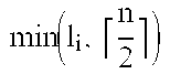
(a′′′, b′′′) 1 k1, k2 = 3, 8 l1, l2 = 1, 1 - The inputs are given in the first column, the sizes of the inputs are given in the second column, and the indices and lengths describing the inputs are given in the third and fourth columns. For this example, a root with a 9-word input is considered. The root's inputs (a,b) are the subarrays of themselves (i.e., a=a[0#9] and b=b[0#9]). Thus, the index and length describing the root's inputs (a,b) are 0 and 9, respectively. The next successor on the path is the mid child of the root with the inputs (a′, b′). Because this successor is a mid branch, its indices and lengths are

- respectively, according to Table 4. After the substitutions k i=k1=0, li=l1=9, and n=9, the indices and lengths describing the inputs of the root's child (a′, b′) are found. These indices and lengths are k1, k2=0,5 and l1, l2=5,4, as seen in Table 5. The size of the inputs (a′, b′) is the new n value, and n=max(l1, l2)=max(5, 4)=5. In this fashion, the indices and lengths describing the inputs (a″, b″) and (a′″, b′″) are found. The inputs (a′″, b′″) comprise (n=1) word. Thus, they are the inputs of the leaf at the end of the path. The indices and lengths describing them are k1, k2=3,8 and l1, l2=1, 1, as seen in Table 5. This means that

- Remember that t′″ denotes the product computed by the leaf at the end of the path and is the product of the leaf's inputs. Thus,

- In this manner, the leaf-product t′″can be expressed in terms of the root's inputs.
- Nonrecursive Functions Derived from KOA
- In this section, exemplary nonrecursive functions KOA2, KOA3, KOA4, KOA5 and KOA6, which multiply 2, 3, 4, 5 and 6-word polynomials respectively, are derived and described. The input size of the functions is derived by analyzing the recursion tree of the KOA.
- Consider two multi-word polynomials that are being multiplied by the KOA. In the recursion tree, these polynomials correspond to the inputs of the root. The root computes their multiplication, benefiting from the computations performed by the other branches (recursive calls). Note that this multiplication, computed by the root, can be expressed as a weighted sum of the leaf-products, as shown in Equation (15). Then, the multiplication of the input polynomials can be performed by computing the weighted sum in Equation (15) without any recursion.
- The leaf-products and their weights are needed to compute the weighted sum in Equation (15). As described above, these parameters can be determined from the root's inputs. As noted, the root's inputs are the multi-word polynomials that are being multiplied. If the size and the words of these inputs are known, the leaf-products and their weights can be obtained through Table 2 and Table 4 in the manner illustrated above in the section concerning recursion trees. A computer program, such as a Maple program, can also be used to perform this process.
- For many input sizes, the weighted sum in Equation (15) is in a particular form, described below, or can be transformed into this particular form through algebraic substitutions. The following proposition and its corollary introduce this form and show how the weighted sums in this form can be computed efficiently.
- Proposition 2: Let lp i and wi for i=0,1, . . . , n−1 denote a set of leaf-products and their weights respectively such that,

- Consequently, t=Σ i=0 n−1 lpiwi is a 2n-word polynomial and can be computed from the leaf-products in the following two steps:
- 1. Compute the (n+1)-word polynomial h from the words of lpi's as follows:
- h[0]=lp0[0],
- h[i]=lp i[0]+lp i−1[1],
- for i=1, . . . , n−1,
- h[n]=lpn−1[1]. (23)
- 2. Compute the words of t from the words of h as follows:
- t[i]=h[i],
- i=0,
- t[i]=t[i−1]+h[i],
- 0<i ≦n−1,
- t[i]=h[i−n+1],
- i=2n−1,
- t[i]=t[i+1]+h[i−n+1],
- n≦i<2n−1. (24)
- The proof of this proposition proceeds as follows. As mentioned before, leaf-products are two-word polynomials. Thus, Σ i=0 n−1 lpizi can be written as:

- The coefficient of z i above is equal to h[i] given in Equation (23) for i=0, . . . , n. Thus, the binary polynomial above is h. In brief, Σi=0 n−1 lpi zi=h=Σi=0 n[i] zi. Then,

- Because z imin+imax=z2n−1, t is a 2n-word polynomial. By using the change of variables k=i+j and l=i, the following can be obtained:
- t=Σk=imin+jmin imaz+jmaz
- Σl=max(imin,k−jmax) min(k−jmin,imax)h[l]z k (27)
- where i min, jmin, imax, jmax are the minimum and maximum values of i and j variables. Because imin=0, jmin=0, imax=n,
j max=n−1,
- Note that t[k], the kth word of t, is the coefficient of the term z k above. Then,

- or equivalently,
- t[k]=Σl=0 kh[l],
- for 0≦k ≦n−1,
- t[k]=Σl=k−n+l nh[l],
- for n≦k≦2n−1. (30)
- We can rewrite the equations above as follows:
- t[k]=h[k]+Σl=0 k−1 h[l],
- for 0≦k≦n−1,
- and
- t[k]=h[k−n+1]+Σl=k−n+2 n h[l],
- for n ≦k≦2n−1. (31)
- For k=i, l=j, the equations above yields the difference equations in Equation (24).
- Corollary : Let lp i and wi for i=0,1, . . . , n−m−1 denote a set of leaf-products and their weights respectively such that,

- Then, t=Σ i=0 n−m−1 lpiwi is a (2n−m)-word polynomial and can be computed from the leaf-products in the following two steps:
- 1. Compute the (n−m+1)-word polynomial h from the words of lpi's as follows:
- h[0]=lp0[0],
- h[i]=lp i[0]+lp i−1[1],
- for i=1, . . . , n−m−1,
- and
- h[n−m]=lp n−m−1[1]. (33)
- 2. Compute the words of t from the words of h as follows:
- t[i]=0,
- 0≦i<m,
- t[i]=h[i−m],
- i=m,
- t[i]=t[i−1]+h[i−m],
- m<i≦n−1,
- t[i]=h[i−n+1],
- i=2n−m−1,
- t[i]=t[i+1]+h[i−n+1],
- n≦i<2n−m−1.
- The proof of the corollary proceeds as follows. The weighted sum Σ i=0 n−m−1 lpiwi can be written as:
- Σi=0 n−m−1 lpiwi=zm
- Σi=0 n−m−1 lpiwi′,
- where w i′=Σj=0 n−m−1 zi+j for i=0,1, . . . , n−m−1. The wi′ terms are in the form given in Equation (22), except that n−m is substituted for n. Thus, the weighted sum Σi=0 n−m−1 lpiwi′ can be computed as shown in
Proposition 2. However, n−m must be substituted for n in the equations given in this proposition. After these substitutions, Equation (23) becomes Equation (33), and Equation (24) becomes - t[i]=h[i],
- i=0,
- t[i]=t[i−1]+h[i],
- 0<i ≦n−m−1,
- t[i]=h[i−n+m+1],
- i=2n−2m−1,
- t[i]=t[i+1]+h[i−n+m+1],
- n−m≦i<2n−2m−1. (35)
- The above equation provides that t=Σ i=0 n−m−1 lpi wi′. However, the desired equation is t=Σi=0 n−m−1 lpiwi. Thus, t must be multiplied by zm to obtain the final result. For this, the index of every word of t is increased by m in the above equation. That is, t[index] is replaced with t[index+m]. This shift in the array representation is the equivalent of multiplying by zm. Also, zeros are inserted into the first m word. After the change of variable i=i+m and some rearrangement, Equation (34) can be obtained.
- FIG. 5 is a flowchart showing generally how the nonrecursive algorithms operate. As shown by the dashed l i nes, the flowchart of FIG. 5 corresponds generally to process block 416 of FIG. 1.
- At
process block 510, the subproduct to be calculated is decomposed into a weighted sum of subproducts having one-word inputs. This decomposition may proceed, for instance, in the manner described above for finding the value and respective weights of the leaf-products from the corresponding recursion tree. Atprocess block 512, algebraic substitutions are performed to identify pairs of identical subproducts. These redundant subproducts are then removed from the weighted sum. The pairs of redundant subproducts can be removed because their sum is zero in GF(2m), thereby reducing the number of XOR operations that need to be performed to obtain the relevant subproduct. Atprocess block 514, subproducts having the form described above inProposition 2 are identified and grouped so that they can be efficiently calculated using the described method. Atprocess block 516, a weighted sum according toProposition 2 is calculated, thereby producing a partial result of the subproduct. As shown in Equation (24), this weighted sum can be obtained using previously calculated intermediate values (e.g., t[i−1] and t[i+1]), which may be stored once they are calculated. This procedure of storing and reusing intermediate values also reduces the number of XOR operations that need to be performed in order to obtain the desired product. Atprocess block 518, the remaining subproducts having one-word inputs are calculated and used to update the partial result. The updated partial result produces the final product, which is returned atprocess block 520. - Although FIG. 5 shows a particular ordering of the processes, the order may vary from embodiment to embodiment. Moreover, the actual implementation of the procedure shown in FIG. 5 may only perform certain ones of the processes. For instance, the actual implementation may comprise code that has already taken into account the pairs of redundant subproducts and removed them from the calculation. Similarly, the subproducts having the special form may already be identified such that the first step performed by the implementation is the calculation of the weighted sum of the subproducts. Further, in certain other implementations, the intermediate values are not stored, but are recalculated.
- Exemplary nonrecursive algorithms that may be used to calculate subproducts having 2-6-word operands are described below.
- Function KOA2
- Let a and b be 2-word polynomials, and their product be t=ab. The product t can be decomposed into the leaf-products, as described above. These leaf-products and their weights are:
i Leaf-Products (lpi) Weights (wi) 0 a[0] b[0] 1 + z 1 a[1] b[1] z + z2 2 (a[0] + a[1]) (b[0] + b[1]) z - Each row above is indexed with i. The ith row contains the ith leaf-product denoted by lp i, and its weight is denoted by wi.
- The product t can be computed as the weighted sum of the leaf-products as in the Equation (15):

- The first two weights can be written as Σ j=0 n−1 zi+j for i=0, . . . , n−1 where n=2. These weights are in the form mentioned in
Proposition 2. Thus, the weighted sum of the first two leaf-products lp0 and lp1 can be computed efficiently, as described in the proposition. But, this weighted sum is only a partial result for t. To obtain t, this partial result must be added to the weighted sum of the remaining leaf-products in the list above (i.e., to (a[0]+a[1]) (b[0]+b[1]) z). - The function below performs the multiplication of 2-word polynomials by computing the weighted sum of the leaf-products.
Inputs: a, b : 2-word polynomials Output: t : 4-word polynomial Temporary: lpi : 2-word polynomials /* Compute the first two leaf-products */ lpi := MULGF2(a[i], b[i]) i = 0, 1 /* Compute h from (23) for n = 2 */ h[0] := lp0[0] h[1] := lp1[0] + lp0[1] h[2] := lp1[1] /* Compute the partial result from (24) for n = 2 */ t[0] := h[0] t[1] := t[0] + h[1] t[3] := h[2] t[2] := t[3] + h[1] /* Compute the remaining leaf-products */ lp3:= MULGF2(a[0] + a[1], b[0] + b[1]) /* Update t with the weighted sum of the remaining leaf-products */ t[1] := t[1] + lp3[0] t[2] := t[2] + lp3[1] - The function above needs 7 word-additions (XOR) and 3 word-multiplications (MULGF2).
- Function KOA3
- Let a and b be 3-word polynomials, and their product be t=ab. The product t can be decomposed into the leaf-products, as described above. As a result of this decomposition, the following leaf-products and weights are obtained:
i Leaf-Products (lpi) Weights (wi) 0 a[0] b[0] 1 + z + z2 + z3 1 a[1] b[1] z + z2 + z3 + z4 2 a[1] b[1] z3 + z4 3 a[2] b[2] z2 + z4 4 (a[0] + a[1]) (b[0] + b[1]) z + z3 5 (a[0] + a[2]) (b[0] + b[2]) z2 + z3 6 (a[0] + a[1] + a[2]) (a[0] + b[1] + b[2]) z3 - Each row above is indexed with i. The ith row contains the ith leaf-product denoted by lp i, and its weight denoted by wi. Note that two of the leaf-products are redundantly the same.
- The value of t can be computed as the weighted sum of the leaf-products as in (15).

- But this does not provide any advantage in terms of computational complexity. Thus, the value of t can be expressed with a modified set of leaf-products and weights so that an efficient scheme for computing the weighted sum can be found. For this purpose, the following substitutions can be made for lp 6=(a[0]+a[1]+a[2])(b[0]+b[1]+b[2]):

- The equality above always holds for arbitrary polynomials over GF(2 m) like a[0, a[1], a[2], b[0], b[1], b[2]. After the substitution, the result is again a weighted sum. Every distinct product in the result is defined as a leaf-product. Let lpi′ denote a particular one of them. This product can appear more than once in the result with different weights. These different weights can be added into a single weight and denoted by wi′:
i Leaf-Products (lp′i) Weights (w′i) 0 a[0] b[0] 1 + z + z2 1 a[1] b[1] z + z2 + z3 2 a[2] b[2] z2 + z3 + z4 3 (a[0] + a[1]) (b[0] + b[1]) z 4 (a[0] + a[2]) (b[0] + b[2]) z2 5 (a[1] + a[2]) (b[1] + b[2]) z3 - As before, each row above contains a leaf-product and its weight, and the corresponding weighted sum gives t:

- The weighted sum of the first three leaf-products in the list above can be written as follows:
- a[0]b[0](1+z+z 2)+a[1]b[1](z+z 2+z3)+a[2]b[2](z 2 +z 3 +z 4) (40)
- The weights above can be written as Σ j=0 n−1 zi+j for i=0, . . . , n−1 where n=3. These weights are in the form mentioned in
Proposition 2, allowing the weighted sum of the first three leaf-products to be computed efficiently as described in the proposition. But, this weighted sum is a partial result for t. To obtain t, this partial result must be added to the weighted sum of the remaining leaf-products in the list above. This weighted sum is: - (a[0]+a[1]) (b[0]b1])z+(a[0]+a[2]) (b[2])z2+(a[1]+a[2]) (b[1]+b [2])z 3 (41)
- The function below performs the multiplication of 3-word polynomials by computing the weighted sum of the leaf-products:
Inputs: a, b : 3-word polynomials Output: t : 6-word polynomial Temporary: lpi : 2-word polynomials /* Compute the first three leaf-products */ lpi := MULGF2(a[i], b[i]) i = 0, ..., 2 /* Compute h from (23) for n = 3 */ h[0] := lp0[0] h[i] := lpi[0] + lpi−l[1] i = 1, ..., 2 h[3] := lp2[1] /* Compute the partial result from (24) for n = 3 */ t[0] := h[0] t[i] := t[i − 1] + h[i] i = 1, 2 t[5] := h[3] t[i] := t[i + 1] + h[i − 2] i = 4, 3 /* Compute the remaining leaf-products */ lp3 := MULGF2(a[0] + a[1], b[0] + b[1]) lp4 := MULGF2(a[1] + a[2], b[1] + b[2]) lp5 := MULGF2(a[0] + a[2], b[0] + b[2]) /* Update t with the weighted sum of the remaining leaf-products in (41) */ t[1] := t[1] + lp3[0] t[2] := t[2] + lp3[1] + lp5[0] t[3] := t[3] + lp5[0] + lp5[1] t[4] := t[4] + lp4[1] - The function above needs 18 word-additions (XOR) and 6 word-multiplications (MULGF2).
- Function KOA4
- Let a and b be 4-word polynomials, and their product be t=ab. The product t can be decomposed into the leaf-products, as described above. These leaf-products and their weights are given below:
i Leaf-Products (lpi) Weights (wi) 0 a[0] b[0] 1 + z + z2 + z3 1 a[1] b[1] z + z2 + z3 + z4 2 a[2] b[2] z2 + z3 + z4 + z5 3 a[3] b[3] z3 + z4 + z5 + z6 4 (a[0] + a[2]) (b[0] + b[2]) z2 + z3 5 (a[1] + a[3]) (b[1] + b[3]) z3 + z4 6 (a[0] + a[1]) (b[0] + b[1]) z2 + z4 7 (a[2] + a[3]) (b[2] + b[3]) z3 + z5 8 (a[0] + a[1] + a[2] + a[3]) (b[0] + z4 b[1] + b[2] + b[3]) - Each row above is indexed with i. The ith row contains the ith leaf-product denoted by lp i and its weight denoted by wi.
- The value of t can be computed as the weighted sum of the leaf-products as in Equation (15).

- The first four weights can be written as Σ j=0 n−1 for i=0, . . . , n−1 where n=4. Also, the fourth and the fifth weights can be written as zm Σj=0 n−m−1 zi+j for i=0, . . . , n−m−1 where n=4 and m=2. These weights are in the forms mentioned in
Proposition 2. Thus, the weighted sum of the first six leaf-products lp0, lp1, lp2, lp3, lp4, and lp5 can be computed efficiently, as described in the proposition. But, this weighted sum is only a partial result for t. To obtain t, this partial result must be added to the weighted sum of the remaining leaf-products in the list above. - The function below performs the multiplication of 4-word polynomials by computing the weighted sum of the leaf-products.
Inputs: a, b : 4-word polynomials Output: t : 8-word polynomial Temporary: lpi : 2-word polynomials /* Compute the first four leaf-products */ lpi := MULGF2(a[i], b[i]) i = 0, ..., 3 /* Compute h from (23) for n = 4 */ h[0] := lp0[0] h[i] := lpi[0] + lpi−l[1] i = 1, ..., 3 h[4] := lp3[1] /* Compute the fourth and fifth leaf-products */ lp4 := MULGF2(a[0] + a[2], b[0] + b[2]) lp5 := MULGF2(a[1] + a[3], b[1] + b[3]) /* Compute h′ from (33) for n = 4 and m = 2 */ h′[0] := lp4[0] h′[1] := lp5[0] + lp4[1] h′[2] := lp5[1] /* Compute the partial result from (24) and (34) for n = 4 and m = 2 */ t[0] := h[0] t[i] := t[i − 1] + h[i] i = 1 t[i] := t[i − 1] + h[i] + h′[i − 2] i = 2, 3 t[7] := h[4] t[i] := t[i + 1] + h[i − 3] i = 6 t[i] := t[i + 1] + h[i − 3] + h′[i − 3] i = 5, 4 /* Compute the remaining leaf-products */ lp6 := MULGF2(a[0] + a[1], b[0] + b[1]) lp7 := MULGF2(a[2] + a[3], b[2] + b[3]) lp8 := MULGF2(a[0] + a[1] + a[2] + a[3], b[0] + b[1] + b[2] + b[3]) /* Update t with the weighted sum of the remaining leaf-products in (41) */ t[1] := t[1] + lp6[0] t[2] := t[2] + lp6[1] t[3] := t[3] + lp8[0] + lp6[0] + lp7[0] t[4] := t[4] + lp8[1] + lp6[1] + lp7[1] t[5] := t[5] + lp7[0] t[6] := t[6] + lp7[1] - The function above needs 38 word-additions (XOR) and 9 word-multiplications (MULGF2). Note that, when lp 6, lp7, and lp8, are computed, 4 XOR operations can be gained at the expense of additional storage.
- Nonrecursive Functions to Multiply Larger Polynomials
- In the previous sections, the functions KOA2, KOA3 and KOA4 were presented for multiplying 2-, 3-, and 4-word polynomials. These functions each compute a weighted sum of leaf-products that yields the output product.
- The leaf-products and their weights are obtained by decomposing the output products into the leaf-products as described above. Sometimes, however, the leaf-products can be redundantly the same and their weighted sum can be simplified by algebraic manipulations. An example of this manipulation was shown with respect to KOA3.
- For the multiplication of the larger polynomials, the same method can be continued to obtain their leaf-products and weights. With the increasing polynomial size, however, removing the redundancies and simplifying the weighted sum of leaf-products becomes more difficult. To overcome this problem, the leaf-products and the weights for the multiplication of the larger polynomials can be derived from the leaf-products and the weights derived for the multiplication of the smaller polynomials. Every time a new set of of the leaf-products and the weights is obtained, they can be optimized. In this fashion, each set of the leaf-products and the weights can be derived from the already optimized leaf-products and the weights. Therefore, only a minor amount of optimization is required in each derivation. This process is more fully explained in the following section.
- Deriving Leaf-Products and Weights for the Multiplication of n-Word Polynomials and for the Multiplication of (n−1)-Word Polynomials
- Let n be an even number. Assume that the product of n/2-word polynomials can be expressed by the following weighted sum:
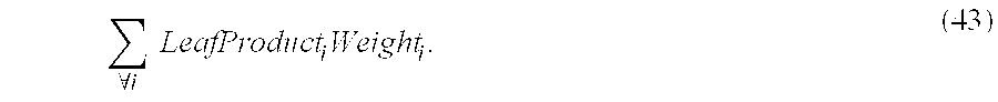
- The leaf-products and the weights above are derived for the multiplication of n/2-word polynomials. From them, the leaf-products and the weights for the multiplication of n and (n−1)-word polynomials can be derived.
- Let t be the product of the n-word polynomials a and b. The product t can be decomposed into three half-sized subproducts according to the following equation (which is similar to equation (14) above):
- t=low (1+z n/2)+mid z n/2+high (z n/2 +z n) (44)
- Note that low, mid and high are the product of n/2-word polynomials:
- low=aLbL
- mid=(a L +a H)(b L +b H)
- high=(aH bH) (45)
- where n/2-word polynomials are:
- a L =a[0#n/2]
- b L =b[0#n/2]
- a H =a[n/2#n/2]
- b H =b[n/2#n/2] (46)
- These terms can be expressed in the weighted sum of Equation (43) as follows:

- where the LeafProduct i's are defined from the words of n/2-word polynomials.
- Note that the product of the n-word polynomials, t, can be expressed with the following weighted sum:

- This weighted sum yields the product of the (n−1)-word polynomials, where the last words of a and b are zero (i.e., a[n−1]=0 and b[n−1]=0).
- Then, the product of the (n−1)-word polynomials can be given by the following weighted sum:

- where a H′=a[n/2#n/2−1] and bH′=b[n/2#n/2−1]. In summary, the leaf-products and the weights for the product of the n-word polynomials can be written as follows:
Leaf-Products Weights 
LeafProducti(aL, bL) Weighti(1 + zn/2) 
LeafProducti(aL + aH, bL + bH) Weightizn/2 
LeafProducti(aH, bH) Weighti(zn/2 + zn) - Similarly, the leaf-products and weights for the product of the (n−1)-word polynomials can be written as follows:
Leaf-Products Weights 
LeafProducti(aL, bL) Weighti(1 + zn/2) 
LeafProducti(aL+ aH′, bL + bH′) Weightizn/2 
LeafProducti(aH′, bH′) Weighti(zn/2 + zn) - Optimizing Leaf-products and Weights
- In general, in one exemplary embodiment, optimizing the leaf-products and weights means that: (1) no leaf-products are redundantly the same; and (2) the weights are in the form mentioned in
Proposition 2 and its corollary. In this sense, the leaf-products and the weight which are derived for the multiplication of n-word polynomials in the previous section are optimum so long as LeafProducti and Weighti are optimum. Further, the leaf-products and the weights which are derived for the multiplication of (n−1)-word polynomials are not optimum, even if LeafProducti and Weighti are optimum. - This can be explained as follows. The leaf-products derived for the multiplication of (n−1)- and n-word polynomials are the same, except that a[n−1]=0 is substituted in the former. The leaf-products are the sum of the words of the inputs a and b. If two leaf-products are the sum of the same words and differ in only a[n−1], there will be no problem for n-word polynomials. However, these two leaf-products look alike for (n−1)-word polynomials. That is, the leaf-products are redundantly the same.
- According to the criteria recited above, Weight i are optimum if

- Three new sets of weights were derived, which can be rewritten as:
- (1+zn/2) Σj=0 n/2−1 zi1+j
- for i1=0, . . . . , n/2−1
- zn/2Σj=0 n/2−1zi2+j
- for i2=0, . . . , n/2−1
- (zn/2+zn) Σj=0 n/2−1 zi3+j
- for i3=0, . . . ,n/2−1
- Note that, (1+z n/2)Σj=0 n/2−1 zi1+j+(z n/2+zn) Σj=0 n/2−1 zi3+j=Σj=0 n/2−1 zi+j i=i1,i3+n/2 Thus, these weights can be written as:
- Σj=0 n−1zi+j
- for i=0, . . . , n−1
- zn/2Σj=0 n/2−1zi+j
- for i=0, . . . , n/2−1
- These weights are in the forms mentioned in Proposition 8 and in its corollary, and thus are optimum. Thus, the leaf-products and the weights derived for n-word polynomials may not need to be optimized when the leaf-products and weights derived for (n/2)-word polynomials have already been optimized. Moreover, the leaf-products and the weights derived for (n−1)-word polynomials may need to be optimized.
- Function KOA5
- Let a and b be 5-word polynomials, and their product be t=ab. The product t can be decomposed into leaf-products in the manner described above. The product t may also be expressed in accordance with the algebraic manipulations described in the previous section. First, zero is substituted for the sixth words a[5) and b[5] in the leaf-product, because the polynomials, which we multiply using the KOA5 function, are of five words, not six. At the end, the following leaf-products and weights are obtained:
i Leaf-Products (lpi) Weights (wi) 0 a[0] b[0] 1 + z + z2 + z3 + z4 + z5 1 a[1] b[1] z + z2 + z3 + z4 + z5 + z6 2 a[2] b[2] z2 + z3 + z4 + z5 + z6 + z7 3 a[3] b[3] z3 + z4 + z5 + z6 + z7 + z8 4 a[4] b[4] z4 + z5 + z6 + z7 + z8 + z9 5 0 z5 + z6 + z7 + z8 + z9 + z10 6 (a[0] + a[1]) (b[0] + b[1]) z + z4 7 (a[0] + a[2]) (b[0] + b[2]) z2 + z5 8 (a[1] + a[3]) (b[1] + b[3]) z3 + z6 9 (a[3] + a[4]) (b[3] + b[4]) z4 + z7 10 (a[3] + 0) (b[3] + 0) z5 + z8 11 (a[4] + 0) (b[4] + 0) z6 + z9 12 (a[0] + a[3]) (b[0] + b[3]) z3 + z4 + z5 13 (a[1] + a[4]) (b[1] + b[4]) z4 + z5 + z6 14 (a[2] + 0) (b[2] + 0) z5 + z6 + z7 15 (a[0] + a[1] + a[3] + a[4]) (b[0] + b[1] + b[3] + b[4]) z4 16 (a([0] + a[2] + a[3] + 0) (b[0] + b[2] + b[3] + 0) z5 17 (a[1] + a[3] + a[4] + 0]) (b[1] + b[3] + b[4] + b[0]) z6 - Each row above is indexed with i. The ith row contains the ith leaf-product denoted by lp i and its weight denoted by wi. The value of t can be computed as the weighted sum of the leaf-products as in Equation (15).

- However, this does not provide any advantage in terms of computational complexity. Instead, the value of t can be expressed with a modified set of leaf-products and weights so that an efficient scheme for computing the weighted sum can be found. For this purpose, the following substitutions can be made for lp 16=(a[0]+a[2]+a[3])(b[0]+b[2]+b[3]) and lp17=(a[1]+a[3]+a[4])(b[1]+b[3]+b[4]):

- After the substitution, the result is again a weighted sum. Every distinct product in the result is defined as a leaf-product. Let lp i′ denote a particular one of them. This product can appear more than once in the result with different weights. Let these different weights be added into a single weight and denoted as wi′. The new leaf-products and weights become:
i Leaf-Products (lp′i) Weights (w′i) 0 a[0] b[0] 1 + z + z2 + z3 + z4 1 a[1] b[1] z + z2 + z3 + z4 + z5 2 a[2] b[2] z2 + z3 + z4 + z5 + z6 3 a[3] b[3] z3 + z4 + z5 + z6 + z7 4 a[4] b[4] z4 + z5 + z6 + z7 + z8 5 (a[0] + a[3]) (b[0] + b[3]) z3 + z4 6 (a[1] + a[4]) (b[1] + b[4]) z4 + z5 7 (a[0] + a[1]) (b[0] + b[1]) z + z4 8 (a[0] + a[2]) (b[0] + b[2]) z2 9 (a[1] + a[2]) (b[1] + b[2]) z3 10 (a[2] + a[3]) (b[2] + b[3]) z5 11 (a[2] + a[4]) (b[2] + b[4]) z6 12 (a[3] + a[4]) (b[3] + b[4]) z4 + z7 13 (a[0] + a[1] + a[3] + a[4]) (b[0] + b[1] + z4 b[3] + b[4]) - The function below performs the multiplication of 5-word polynomials, by computing the weighted sum of the leaf-products.
Inputs: a, b : 5-word polynomials Output: t : 10-word polynomial Temporary: lpi : 2-word polynomials /* Compute the first four leaf-products */ lpi := MULGF2(a[i], b[i]) i = 0, ..., 4 /* Compute h from (23) for n = 5 */ h[0] := lp0[0] h[i] := lpi[0] + lpi−l[1] i = 1, ..., 4 h[5] := lp4[1] /* Compute the fourth and fifth leaf-products */ lp5 := MULGF2(a[0] + a[3], b[0] + b[3]) lp6 := MULGF2(a[1] + a[4], b[1] + b[4]) /* Compute h′ from (33) for n = 5 and m = 3 */ h′[0] := lp5[0] h′[1] := lp6[0] + lp5[1] h′[2] := lp6[1] /* Compute the partial result from (24) and (34) for n = 5 and m = 3 */ t[0] := h[0] t[i] := t[i − 1] + h[i] i = 1, 2 t[i] := t[i − 1] + h[i] + h′[i − 3] i = 3, 4 t[9] := h[5] t[i] := t[i + 1] + h[i − 4] i = 8, 7 t[i] := t[i + 1] + h[i − 4] + h′[i − 4] i = 6, 5 /* Compute the remaining leaf-products */ lp7 := MULGF2(a[0] + a[1], b[0] + b[1]) lp8 := MULGF2(a[0] + a[2], b[0] + b[2]) lp9 := MULGF2(a[1] + a[2], b[1] + b[2]) lp10 := MULGF2(a[2] + a[3], b[2] + b[3]) lp11 := MULGF2(a[2] + a[4], b[2] + b[4]) lp12 := MULGF2(a[3] + a[4], b[3] + b[4]) lp13 := MULGF2(a[0] + a[1] + a[3] + a[4], b[0] + b[1] + b[3] + b[4]) /* Update t with the weighted sum of the remaining leaf- products */ t[1] := t[1] + lp7[0] t[2] := t[2] + lp7[1] + lp8[0] t[3] := t[3] + lp9[0] + lp8[1] t[4] := t[4] + lp9[1] + lp13[0] + lp7[0] + lp12[0] t[5] := t[5] + lp10[0] + lp13[1] + lp7[1] + lp12[1] t[6] := t[6] + lp10[1] + lp11[0] t[7] := t[7] + lp12[0] + lp11[1] t[8] := t[8] + lp12[1] - The function above needs 57 word-additions (XOR) and 14 word-multiplications (MULGF2). Note that when lp 7, lp12, and lp13 are computed, 4 XOR operations are gained at the expense of additional storage.
- Function KOA6
- Let a and b be 6-word polynomials, and their product be t=ab. The t can be decomposed into the leaf-products as follows:
i Leaf-Products (lpi) Weights (wi) 0 a[0] b[0] 1 + z + z2 + z3 + z4 + z5 1 a[1] b[1] z + z2 + z3 + z4 + z5 + z6 2 a[2] b[2] z2 + z3 + z4 + z5 + z6 + z7 3 a[3] b[3] z3 + z4 + z5 + z6 + z7 + z8 4 a[4] b[4] z4 + z5 + z6 + z7 + z8 + z9 5 a[5] b[5] z5 + z6 + z7 + z8 + z9 + z10 6 (a[0] + a[1]) (b[0] + b[1]) z + z4 7 (a[0] + a[2]) (b[0] + b[2]) z2 + z5 8 (a[1] + a[3]) (b[1] + b[3]) z3 + z6 9 (a[3] + a[4]) (b[3] + b[4]) z4 + z7 10 (a[3] + a[5]) (b[3] + b[5]) z5 + z8 11 (a[4] + a[5]) (b[4] + b[5]) z6 + z9 12 (a[0] + a[3]) (b[0] + b[3]) z3 + z4 + z5 13 (a[1] + a[4]) (b[1] + b[4]) z4 + z5 + z6 14 (a[2] + a[5]) (b[2] + b[5]) z5 + z6 + z7 15 (a[0] + a[1] + a[3] + a[4]) (b[0] + b[1] + b[3] + b[4]) z4 16 (a[0] + a[2] + a[3] + a[5]) (b[0] + b[2] + b[3] + b[5]) z5 17 (a[1] + a[3] + a[4] + a[5]) (b[1] + b[3] + b[4] + b[5]) z6 - The function below performs the multiplication of 6-word polynomials, by computing the weighted sum of the leaf-products.
Inputs: a, b : 6-word polynomials Output: t : 12-word polynomial Temporary: lpi : 2-word polynomials /* Compute the first six leaf-products */ lpi := MULGF2(a[i], b[i]) i = 0, ..., 5 /* Compute h from (23) for n = 6 */ h′[0] := lp0[0] h′[i] := lpi[0] + lPi−l[1] i = 1, ..., 5 h′[6] := lp5[1] /* Compute the 12th, 13th and 14th leaf-products */ lp12 := MULGF2(a[0] + a[3], b[0] + b[3]) lp13 := MULGF2(a[1] + a[4], b[1] + b[4]) lp14 := MULGF2(a[2] + a[5], b[2] + b[5]) /* Compute h′ from (33) for n = 6 and m = 3 */ h′[0] := lp12[0] h′[1] := lp13[0] + lp12[1] h′[2] := lp14[0] + lp13[1] h′[3] := lp14[1] /* Compute the partial result from (24) and (34) for n = 6 and m = 3 */ t[0] := h[0] t[i] := t[i − 1] + h[i] i = 1, 2 t[i] := t[i − 1] + h[i] + h′[i − 3] i = 3, 4, 5 t[11] := h[6] t[i] := t[i + 1] + h[i − 5] i = 10, 9 t[i] := t[i + 1] + h[i − 5] + h′[i − 5] i = 8, 7, 6 /* Compute the remaining leaf-products */ lp6 := MULGF2(a[0] + a[1], b[0] + b[1]) lp7 := MULGF2(a[0] + a[2], b[0] + b[2]) lp8 := MULGF2(a[1] + a[3], b[1] + b[3]) lp9 := MULGF2(a[3] + a[4], b[3] + b[4]) lp10 := MULGF2(a[3] + a[5], b[3] + b[5]) lp11 := MULGF2(a[4] + a[5], b[4] + b[5]) lp15 := MULGF2(a[0] + a[1] + a[3] + a[4], b[0] + b[1] + b[3] + b[4]) lp16 := MULGF2(a[0] + a[2] + a[3] + a[5], b[0] + b[2] + b[3] + b[5]) lp17 := MULGF2(a[1] + a[3] + a[4] + a[5], b[1] + b[3] + b[4] + b[5]) /* Update t with the weighted sum of the remaining leaf- products */ t[1] := t[1] + lp6[0] t[2] := t[2] + lp6[1] + lp7[0] t[3] := t[3] + lp8[0] + lp7[1] t[4] := t[4] + lp8[1] + lp9[0] + lp6[0] + lp15[0] t[5] := t[5] + lp10[0] + lp9[1] + lp6[1] + lp15[1] + lp16[0] t[6] := t[6] + lp10[1] + lp11[0] + lp8[0] + lp17[0] + lp16[1] t[7] := t[7] + lp9[0] + lp11[1] + lp8[1] + lp17[1] t[8] := t[8] + lp9[1] + lp10[0] t[9] := t[9] + lp11[0] + lp10[1] t[10] := t[10] + lp11[1] - The function above needs 81 word-additions (XOR) and 18 word-multiplications (MULGF2). Note that when the remaining leaf-products are computed and the result updated with their weighted sum, 9 XOR operations are gained. Additional storage, however, may be needed to achieve this gain.
- Performance Analysis
- The performance of the disclosed GF(2 m) multiplication methods mainly depend on the performance of the particular LKOA implemented. The cost of the modulo reduction operation is typically less significant if a trinomial or pentanomial is selected as the irreducible polynomial. In the following table, the number of XOR and MULGF2 operations required to multiply polynomials having a size between 2 and 6 words using standard multiplication, the KOA, and the LKOA described above is given.
Polynomial Size n 2 3 4 5 6 XOR Standard 4 12 24 40 60 KOA 8 28 40 84 108 LKOA 7 18 38 57 81 MULGF2 Standard 4 9 16 25 36 KOA 3 7 9 17 21 LKOA 3 6 9 14 18 - As seen in Table 6, the standard multiplication needs n 2 MULGF2 operations to compute the partial products and needs 2n(n−1) XOR operations to combine these partial products. The number of XOR and MULGF2 operations required for the KOA is calculated using a computer program, such as a Maple program. As seen from Table 6, the LKOA and the KOA need more XOR operations. However, the LKOA and the KOA need fewer MULGF2 operations than the standard multiplication. Because the emulation of MULGF2 is very costly, the LKOA and the KOA outperform the standard multiplication.
- In comparison to other methods, GF(2 m) multiplication with the LKOA is more efficient, can be implemented in software in a computer-based environment, does not require a look-up table, and does not have a restriction on the field size m. Although the LKOA may require extra code size, the overall code size is still very reasonable. For example, the code for the particular implementation discussed above in the C programming language requires at most 5 kbytes.
- A multiplication method using both the LKOA and the KOA for calculating polynomials in GF(2 m) may be implemented in software. Trinomials and pentanomials may be used for the reduction procedure that follows multiplication. Table 7 gives the timing results for two particular implementations for multiplying GF(2m): (1) the LKOA; and (2) the KOA.
TABLE 7 Timing results for GF(2m) multiplication by the KOA and the LKOA Field Size m 163 211 233 283 Field Size in words (n = [m/32]) 6 7 8 9 GF(2m) multiplication by KOA 9.2 μs 10.2 μs 10.6 μs 18.8 μs GF(2m) multiplication by LKOA 5.0 μs 6.3 μs 6.7 μs 10.3 μs - The multiplication time for the finite fields GF(2 163), GF(2211), GF(2233), and GF(2283), which are commonly used in the elliptic curve cryptography, were measured. The particular platform used in the measurement was a 450-MHZ Pentium II machine with 256 Mbyte RAM. The timing results show that the LKOA is nearly two times faster than the KOA for GF(2m) multiplication.
- The operation of one of the nonrecursive algorithms is illustrated in the following example and in FIGS. 6 through 8. In particular, FIGS. 6 through 8 illustrate the operation of the KOA3 algorithm by relating it to the recursion tree of FIG. 2. In this example, two polynomials “110110” and “100101” (i.e., 1+x+x 3+x4 and 1+x3+x5) are multiplied together. Both polynomials comprise three two-bit words. Thus, the operand size is n=3, and the word size is w=2. Let a
denote 110110 and a[i] denote the ith bit of 110110. Also, let b denote 100101 and b[i] denote the ith digit of 100101. - The first process in the KOA3 algorithm is to compute the first three leaf-products lp 0, lp1, and lp2. In particular, these subproducts are lp0=11*10=1100, lp1=01*01=0010, and lp2=10*01=0100. As shown in F these subproducts correspond to branches of the related recursion tree. In particular, lp0 corresponds to branch 231,
lp 1 corresponds tobranches - The second process in the KOA3 algorithm is to compute h from these leaf-products according to Equation (23). In particular, h is computed as follows:
- h[0]:=lp0[0]
- h[i]:=lp i[0]+lp i−1[1]
- i=1, . . . , 2
- h[3]:=lp2[1]
- FIG. 6 shows this computation as a weighted sum of word-shifted versions of the leaf-products.
- The third process in the KOA3 algorithm is to compute the partial result according to the following weighted sum:
- t[0]:=h[0]
- t[i]:=t[i−1]+h[i]
- for i=1,2
- t[5]:=h[3]
- t[i]:=t[i+1]+h[i−2]
- for i=4,3
- FIG. 7 illustrates this computation as a weighted sum of the individual words from h combined with previously calculated terms. For instance, t[0] is calculated first. Then, t[l] is calculated from h(1] and the previously calculated value of t[0]. Similarly, t[5] is calculated after t[0] through t[2]. Then, t[4] is calculated as the sum of h[4] and the previously calculated value of t[5]. In this manner, the partial result is determined by storing and reusing previously calculated values, thereby reducing the number of XOR operations required to obtain the partial result.
- The fourth process in the KOA3 algorithm is to determine the remaining leaf-products lp 3, lp4, and lp5. In particular, these subproducts are lp3=10*11=1100, lp4=01*11=0110, and lp5=11*00 =0000. As shown in FIG. 8, these subproducts correspond to branches of the related recursion tree. In particular, lp3 corresponds to branch 232, lp4 corresponds to branch 234, and lp5 corresponds to branch 235. Note that lp5 no longer corresponds precisely to branch 235, but has instead been modified through the algebraic substitutions recited above to comprise the subproduct (a[1]+a[2])(b[1]+b[2]). As more fully discussed above, the algebraic substitutions can performed to maximize the number of one-word subproducts having weights in the form Σj=0 n−1 zi+j for i=0, . . . , n−1, which can be efficiently calculated.
- The fifth process in the KOA3 algorithm is to update the partial result with the remaining leaf-products. In particular, this update is performed as follows:
- t[1]:=t[1]+lp 3[0]
- t[2]:=t[2]+lp 3[1]+lp 5[0]
- t[3]:=t[3]+lp 5[0]+lp 5[1]
- t[4]:=t[4]+lp 4[1]
- FIG. 8 illustrates this computation as a weighted sum of word-shifted versions of the remaining leaf-products. As a result of this computation, the final result is obtained. The final result may then be used as part of a recursive algorithm to compute the product of operands having a larger word size.
- Applications of the LKOA
- The methods described above may be used in a variety of different applications wherein multiplication of multi-precision numbers is performed. For example, the methods may be used in a software program that performs arbitrary-precision arithmetic (e.g., Mathematica) or in other specialized or general-purpose software implementations. Additionally, the methods may be used in the field of cryptography, which often involves the manipulation of large multi-precision numbers. For example, the methods may be used to at least partially perform the calculation of a variety of different cryptographic parameters. These cryptographic parameters may include, for instance, a public key, a private key, a ciphertext, a plaintext, a digital signature, or a combination of these parameters. Cryptographic systems that may benefit from the disclosed methods and apparatus include, but are not limited to, systems using the RSA algorithm, the Diffie-Hellman key exchange algorithm, the Digital Signature Standard (DSS), elliptic curves, the Elliptic Curve Digital Signature Algorithm (ECDSA), or other algorithms.
- In one particular implementation, the methods are used, at least in part, to generate and verify a key pair or to generate and verify a signature according to the ECDSA. For example, the methods may be used to compute Q=dG during the key pair generation process, wherein Q is a public key, d is a private key, and G is a base point. Moreover, the methods may be used to verify that nQ=O during the key pair verification process, wherein n is the order of the point G, and O is the point at infinity of the elliptic curve. Similarly, the methods may be used to compute kG=(x 1,y1), wherein k is a random or pseudorandom integer, and (x1, y1) are points on an elliptic curve. The methods may similarly be used to calculate the related modular, inverse modular, and hash functions during the signature generation and verification processes.
- Any of the methods described above may be implemented in a number of different hardware and/or software environments. FIG. 11 shows a block diagram of one exemplary general hardware implementation. More particularly, FIG. 9 shows a multiplying apparatus 900 (e.g., a computer) that includes a processor 910 (e.g., a microprocessor), memory 912 (e.g., RAM or ROM) and an
input data path 914. Any one of the multiplication methods described above may be stored in the memory or on a computer-readable medium (e.g., hard disk, CD-ROM, DVD, floppy disk, RAM, ROM) that is separate from thememory 912 and accessible by theprocessor 910 before or during execution of the algorithm. During operation, the input operands (e.g., polynomials) may be supplied via theinput data path 914 or by thememory 912. Theprocessor 910 and thememory 912 are coupled together via thedata paths 916, which enable the various read and write operations performed during the algorithm. The final product computed by theprocessor 910 may be output from the processor onoutput data path 916 or stored in thememory 912 for later use. The details of this general hardware implementation are omitted. - As noted, the disclosed methods may be used in cryptography to help compute a variety of cryptographic parameters using multi-precision multiplication. FIG. 10 shows a block diagram of a general
cryptographic apparatus 940 that may be used to multiply two operands to produce a cryptographic parameter. Theapparatus 940 includes acryptographic processor 950 used to perform the algorithm;memory 952 used to store the operands, the intermediate results, and computer-executable instructions for performing the algorithm; and aninput data path 954. Theapparatus 940 operates much like the apparatus described in FIG. 9, but produces a cryptographic parameter at itsoutput 956. The cryptographic parameter may be related to or constitute a portion of a public key, private key, ciphertext, plaintext, digital signature, or some combination thereof. The parameter may also constitute a number of other values used in cryptography. Thecryptographic apparatus 940 may be included in a variety of security applications. For instance, theapparatus 940 may be included in a secure transaction server used for financial transactions, confidential record storage, SmartCards, and cell phones. - In view of the many possible implementations, it will be recognized that the illustrated embodiments include only examples and should not be taken as a limitation on the scope of the disclosed technology. Instead, the invention is intended to encompass all alternatives, modifications, and equivalents as may be included within the spirit and scope of the technology defined by the following claims.
Claims (39)
1. A method of multiplying a first polynomial and a second polynomial over GF(2m), comprising:
representing the first polynomial and the second polynomial as an array of n words, wherein n is an integer,
using a recursive algorithm to decompose a multiplication of the first polynomial and the second polynomial into a weighted sum of iteratively smaller subproducts; and
using a nonrecursive algorithm to complete the multiplication when a size of the smaller subproducts is less than or equal to a predetermined size, the predetermined size being at least two words.
2. The method of claim 1 , wherein the predetermined size is six words.
3. The method of claim 1 , wherein the recursive multiplication algorithm is a Karatsuba-Ofman algorithm.
4. The method of claim 1 , wherein the step of using a nonrecursive multiplication algorithm includes the step of excluding pairs of redundant subproducts.
5. The method of claim 1 , wherein the nonrecursive multiplication algorithm stores and reuses previously calculated intermediate values to determine subsequent intermediate values.
6. The method of claim 5 , wherein the previously calculated intermediate values are used to determine a weighted sum of subproducts having weights z of the form Σj=0 n−1 zi+j for i=0, . . . , n−1, wherein i and j are index integers.
7. The method of claim 6 , wherein the subproducts having weights of Σj=0 n−1 zi+j for i=0, . . . , n−1 are one-word subproducts lpi of a corresponding recursion tree, and the weighted sum of the subproducts is denoted as t, the method further comprising:
calculating a (n+1)-word polynomial h from the one-word subproducts lpi, wherein,
h[0]=lp0[0],h[i]=lp i[0]+lp i−1[1], for i=1, n−m−1,h[n−m]=lp n−m−1[1],
where h[i] is the ith word of h and m−1 is a degree of the first polynomial; and
calculating a weighted sum t from words of h, wherein:
t[i]=h[i], for i=0,t[i]=t[i−1]+h[i], for 0<i≦n−1,t[i]=h[i−n+1], for i=2n−1,t[i]=t[i+1]+h[i−n+1], for n≦i<2n−1,
where t[i] is the ith word of t.
8. The method of claim 1 , wherein at least one of the first and the second polynomials corresponds to at least a portion of a private key, and a product of the first polynomial and the second polynomial corresponds to a public key.
9. The method of claim 1 , wherein the first polynomial and the second polynomial are cryptographic parameters and the multiplication is associated with signature generation.
10. The method of claim 9 , wherein the signature generation is associated with an elliptic curve digital signature.
11. The method of claim 1 , wherein the first polynomial and the second polynomial are associated with cryptographic parameters and the multiplication is associated with signature verification.
12. The method of claim 11 , wherein the signature verification is associated with an elliptic curve digital signature.
13. A computer-readable medium, comprising instructions for performing the method of claim 1 .
14. A method of multiplying a first polynomial and a second polynomial over GF(2m):
representing the first polynomial and the second polynomial as n words, wherein n is an integer greater than one;
determining a partial result by calculating a weighted sum of one-word subproducts having weights z of a form Σj=0 n−1 zi+j for i=0, . . . , n−1, wherein i and j are index integers; and
updating the partial result by adding remaining one-word subproducts.
15. The method of claim 14 , further comprising identifying and excluding pairs of redundant one-word subproducts.
16. The method of claim 14 , wherein the determining the partial result comprises:
storing intermediate calculations in a memory; and
reusing the stored intermediate calculations.
17. The method of claim 14 , wherein the one-word subproducts are denoted as leaf-products lpi, and the determining the partial result comprises:
calculating a (n+1)-word polynomial h from the leaf-products lpi, wherein,
h[0]=lp0[0],h[i]=lp i[0]+lp i−1[1], for i=1, . . . , n−m−1,h[n−m]=lp n−m−1[1],
where h[i] is the ith word of h and m−1 is a degree of the first polynomial; and
calculating a weighted sum t from words of h, wherein:
t[i]=h[i], for i=0,t[i]=t[i−1]+h[i], for 0<i≦n−1,t[i]=h[i−n+1], for i=2n−1,t[i]=t[i+1]+h[i−n+1], for n≦i<2n−1,
where t[i] is the ith word of t.
18. The method of claim 14 , wherein at least one of the first and the second polynomials is associated with a private key, and a product of the first polynomial and the second polynomial is associated with a public key.
19. The method of claim 14 , wherein the first polynomial and the second polynomial are cryptographic parameters and the multiplication is associated with signature generation.
20. The method of claim 19 , wherein the signature generation is associated with an elliptic curve digital signature.
21. The method of claim 14 , wherein the first polynomial and the second polynomial are cryptographic parameters and the multiplication is associated with signature verification.
22. The method of claim 21 , wherein the signature verification process is associated with an elliptic curve digital signature.
23. A computer-readable medium, comprising instructions for performing the method of claim 14 .
24. A method of determining an algorithm for multiplying a first polynomial and a second polynomial over GF(2m):
decomposing a product of the first polynomial and the second polynomial into a weighted sum of one-word subproducts;
identifying pairs of redundant one-word subproducts; and
removing the pairs of redundant one-word subproducts from the weighted sum, thereby obtaining a revised weighted sum.
25. The method of claim 24 , wherein the first polynomial and the second polynomial have n−1 words, where n is an even integer, and wherein the first and the second polynomials are padded with zeros such that the first polynomial and the second polynomial can be represented as n words.
26. The method of claim 24 , wherein the zero-padded words of the first and the second polynomials are excluded from the revised weighted sum.
27. The method of claim 24 , further comprising identifying the one-word subproducts having weights z of a form Σj=0 n−1 zi+j for i=0, . . . , n−1 through algebraic substitutions, wherein i and j are index integers, and n is a number of words in the first and second polynomials.
28. The method of claim 27 , further comprising calculating a weighted sum of the one-word subproducts having weights of Σj=0 n−1 zi+j for i=0, . . . , n−1 by storing and reusing intermediate calculations.
29. A nonrecursive algorithm determined by the method of claim 24 .
30. A computer-readable medium, comprising instructions for performing the nonrecursive algorithm of claim 24 .
31. A cryptographic method, comprising:
receiving a first operand and a second operand, the first operand and the second operand representing a first polynomial over GF(2m) and a second polynomial over GF(2m);
multiplying the first operand and the second operand in a multiplication process, the multiplication process comprising:
using a recursive algorithm to reduce the multiplication of the first operand and the second operand into a weighted sum of smaller subproducts; and
using a nonrecursive algorithm to multiply the smaller subproducts when a size of the smaller subproducts is less than or equal to a predetermined size, the predetermined size being at least two words; and
outputting a cryptographic parameter associated with the multiplication.
32. The method of claim 31 , wherein the predetermined size is six words.
33. The method of claim 31 , wherein the recursive multiplication algorithm is a Karatsuba-Ofman algorithm.
34. The method of claim 31 , wherein the nonrecursive multiplication algorithm excludes pairs of redundant subproducts.
35. The method of claim 31 , wherein the nonrecursive multiplication algorithm uses previously calculated, stored weighted sums to determine subsequent weighted sums.
36. The method of claim 31 , wherein at least one of the operands corresponds to a private key, and the cryptographic parameter is a public key.
37. The method of claim 31 , wherein the cryptographic parameter is used in digital signature generation or digital signature verification.
38. The method of claim 37 , wherein the signature generation is associated with an elliptic curve digital signature.
39. An apparatus for multiplying a first polynomial and a second polynomial over GF(2m), comprising:
means for receiving the first polynomial and the second polynomial;
means for storing the first polynomial and the second polynomial as a series of words;
means for recursively multiplying the first polynomial and the second polynomial by dividing the stored first and second polynomials into multiple smaller subproducts until an input size of the subproducts is less than a predetermined size;
means for nonrecursively multiplying the subproducts when the size of the inputs is less than the predetermined size, the predetermined size being at least two words;
means for outputting the product of the first polynomial and the second polynomial.
Priority Applications (1)
| Application Number | Priority Date | Filing Date | Title |
|---|---|---|---|
| US10/636,326 US7447310B2 (en) | 2002-08-06 | 2003-08-06 | Lean multiplication of multi-precision numbers over GF(2m) |
Applications Claiming Priority (3)
| Application Number | Priority Date | Filing Date | Title |
|---|---|---|---|
| US40157402P | 2002-08-06 | 2002-08-06 | |
| US41920402P | 2002-10-16 | 2002-10-16 | |
| US10/636,326 US7447310B2 (en) | 2002-08-06 | 2003-08-06 | Lean multiplication of multi-precision numbers over GF(2m) |
Publications (2)
| Publication Number | Publication Date |
|---|---|
| US20040109561A1 true US20040109561A1 (en) | 2004-06-10 |
| US7447310B2 US7447310B2 (en) | 2008-11-04 |
Family
ID=32475363
Family Applications (1)
| Application Number | Title | Priority Date | Filing Date |
|---|---|---|---|
| US10/636,326 Expired - Fee Related US7447310B2 (en) | 2002-08-06 | 2003-08-06 | Lean multiplication of multi-precision numbers over GF(2m) |
Country Status (1)
| Country | Link |
|---|---|
| US (1) | US7447310B2 (en) |
Cited By (8)
| Publication number | Priority date | Publication date | Assignee | Title |
|---|---|---|---|---|
| US20040098440A1 (en) * | 2002-08-06 | 2004-05-20 | The State Of Oregon Acting By And Through The State Board Of Higher Education On Behalf Of | Multiplication of multi-precision numbers having a size of a power of two |
| US20060161613A1 (en) * | 2005-01-05 | 2006-07-20 | Lg Electronics Inc. | Method and apparatus for arithmatic operation of processor |
| DE102005028662A1 (en) * | 2005-03-04 | 2006-09-07 | IHP GmbH - Innovations for High Performance Microelectronics/Institut für innovative Mikroelektronik | Polynom multiplication calculating method e.g. for elliptical curve cryptography, making available coefficients with two polynomials each polynomial fragmented into two or more fragments, being operands partial multiplication |
| US7363336B1 (en) | 2004-03-19 | 2008-04-22 | Microsoft Corporation | Six-term Karatsuba-variant calculator |
| US20090157790A1 (en) * | 2007-12-15 | 2009-06-18 | Vinodh Gopal | Method and apparatus for multiplying polynomials with a prime number of terms |
| US7765252B1 (en) * | 2004-03-19 | 2010-07-27 | Microsoft Corporation | Five-term karatsuba-variant calculator |
| US10474431B2 (en) * | 2014-11-07 | 2019-11-12 | IHP GmbH—Innovations for High Performance Microelectronics/Leibniz-Institut fur innovative Mikroelektronik | Device and method for multiplication for impeding side-channel attacks |
| CN113485751A (en) * | 2021-06-30 | 2021-10-08 | 海光信息技术股份有限公司 | Method for performing Galois field multiplication, arithmetic unit and electronic device |
Families Citing this family (45)
| Publication number | Priority date | Publication date | Assignee | Title |
|---|---|---|---|---|
| US8620980B1 (en) | 2005-09-27 | 2013-12-31 | Altera Corporation | Programmable device with specialized multiplier blocks |
| US8266198B2 (en) | 2006-02-09 | 2012-09-11 | Altera Corporation | Specialized processing block for programmable logic device |
| US8266199B2 (en) | 2006-02-09 | 2012-09-11 | Altera Corporation | Specialized processing block for programmable logic device |
| US8301681B1 (en) | 2006-02-09 | 2012-10-30 | Altera Corporation | Specialized processing block for programmable logic device |
| US8386550B1 (en) | 2006-09-20 | 2013-02-26 | Altera Corporation | Method for configuring a finite impulse response filter in a programmable logic device |
| US8386553B1 (en) | 2006-12-05 | 2013-02-26 | Altera Corporation | Large multiplier for programmable logic device |
| US7930336B2 (en) | 2006-12-05 | 2011-04-19 | Altera Corporation | Large multiplier for programmable logic device |
| US8650231B1 (en) | 2007-01-22 | 2014-02-11 | Altera Corporation | Configuring floating point operations in a programmable device |
| US8645450B1 (en) | 2007-03-02 | 2014-02-04 | Altera Corporation | Multiplier-accumulator circuitry and methods |
| US7991162B2 (en) * | 2007-09-14 | 2011-08-02 | University Of Ottawa | Accelerating scalar multiplication on elliptic curve cryptosystems over prime fields |
| US8144864B2 (en) * | 2007-12-28 | 2012-03-27 | Intel Corporation | Method for speeding up the computations for characteristic 2 elliptic curve cryptographic systems |
| US8959137B1 (en) | 2008-02-20 | 2015-02-17 | Altera Corporation | Implementing large multipliers in a programmable integrated circuit device |
| US20110106872A1 (en) * | 2008-06-06 | 2011-05-05 | William Hasenplaugh | Method and apparatus for providing an area-efficient large unsigned integer multiplier |
| US8307023B1 (en) | 2008-10-10 | 2012-11-06 | Altera Corporation | DSP block for implementing large multiplier on a programmable integrated circuit device |
| US8706790B1 (en) | 2009-03-03 | 2014-04-22 | Altera Corporation | Implementing mixed-precision floating-point operations in a programmable integrated circuit device |
| US8645449B1 (en) | 2009-03-03 | 2014-02-04 | Altera Corporation | Combined floating point adder and subtractor |
| US8468192B1 (en) * | 2009-03-03 | 2013-06-18 | Altera Corporation | Implementing multipliers in a programmable integrated circuit device |
| US8650236B1 (en) | 2009-08-04 | 2014-02-11 | Altera Corporation | High-rate interpolation or decimation filter in integrated circuit device |
| US8412756B1 (en) | 2009-09-11 | 2013-04-02 | Altera Corporation | Multi-operand floating point operations in a programmable integrated circuit device |
| US8396914B1 (en) | 2009-09-11 | 2013-03-12 | Altera Corporation | Matrix decomposition in an integrated circuit device |
| US8539016B1 (en) | 2010-02-09 | 2013-09-17 | Altera Corporation | QR decomposition in an integrated circuit device |
| US20110005757A1 (en) * | 2010-03-01 | 2011-01-13 | Jeff Hebert | Device and method for flowing back wellbore fluids |
| US8601044B2 (en) | 2010-03-02 | 2013-12-03 | Altera Corporation | Discrete Fourier Transform in an integrated circuit device |
| US8484265B1 (en) | 2010-03-04 | 2013-07-09 | Altera Corporation | Angular range reduction in an integrated circuit device |
| US8510354B1 (en) | 2010-03-12 | 2013-08-13 | Altera Corporation | Calculation of trigonometric functions in an integrated circuit device |
| US8539014B2 (en) | 2010-03-25 | 2013-09-17 | Altera Corporation | Solving linear matrices in an integrated circuit device |
| US8862650B2 (en) | 2010-06-25 | 2014-10-14 | Altera Corporation | Calculation of trigonometric functions in an integrated circuit device |
| US8589463B2 (en) | 2010-06-25 | 2013-11-19 | Altera Corporation | Calculation of trigonometric functions in an integrated circuit device |
| US8577951B1 (en) | 2010-08-19 | 2013-11-05 | Altera Corporation | Matrix operations in an integrated circuit device |
| US8645451B2 (en) | 2011-03-10 | 2014-02-04 | Altera Corporation | Double-clocked specialized processing block in an integrated circuit device |
| US9600278B1 (en) | 2011-05-09 | 2017-03-21 | Altera Corporation | Programmable device using fixed and configurable logic to implement recursive trees |
| US8812576B1 (en) | 2011-09-12 | 2014-08-19 | Altera Corporation | QR decomposition in an integrated circuit device |
| US8949298B1 (en) | 2011-09-16 | 2015-02-03 | Altera Corporation | Computing floating-point polynomials in an integrated circuit device |
| US9053045B1 (en) | 2011-09-16 | 2015-06-09 | Altera Corporation | Computing floating-point polynomials in an integrated circuit device |
| US8762443B1 (en) | 2011-11-15 | 2014-06-24 | Altera Corporation | Matrix operations in an integrated circuit device |
| US8543634B1 (en) | 2012-03-30 | 2013-09-24 | Altera Corporation | Specialized processing block for programmable integrated circuit device |
| US9098332B1 (en) | 2012-06-01 | 2015-08-04 | Altera Corporation | Specialized processing block with fixed- and floating-point structures |
| US8996600B1 (en) | 2012-08-03 | 2015-03-31 | Altera Corporation | Specialized processing block for implementing floating-point multiplier with subnormal operation support |
| US9207909B1 (en) | 2012-11-26 | 2015-12-08 | Altera Corporation | Polynomial calculations optimized for programmable integrated circuit device structures |
| US9189200B1 (en) | 2013-03-14 | 2015-11-17 | Altera Corporation | Multiple-precision processing block in a programmable integrated circuit device |
| US9348795B1 (en) | 2013-07-03 | 2016-05-24 | Altera Corporation | Programmable device using fixed and configurable logic to implement floating-point rounding |
| US9417848B2 (en) * | 2014-03-28 | 2016-08-16 | Storart Technology Co. Ltd. | Serial multiply accumulator for galois field |
| CN104065478B (en) * | 2014-06-18 | 2017-07-14 | 天津大学 | Polynomial modulo multiplication coprocessor based on lattice cryptosystem |
| US9684488B2 (en) | 2015-03-26 | 2017-06-20 | Altera Corporation | Combined adder and pre-adder for high-radix multiplier circuit |
| US10942706B2 (en) | 2017-05-05 | 2021-03-09 | Intel Corporation | Implementation of floating-point trigonometric functions in an integrated circuit device |
Citations (31)
| Publication number | Priority date | Publication date | Assignee | Title |
|---|---|---|---|---|
| US4037093A (en) * | 1975-12-29 | 1977-07-19 | Honeywell Information Systems, Inc. | Matrix multiplier in GF(2m) |
| US4435823A (en) * | 1980-12-29 | 1984-03-06 | Harris Corporation | Adaptive equalizer capable of linear and nonlinear weighting |
| US4754421A (en) * | 1985-09-06 | 1988-06-28 | Texas Instruments Incorporated | Multiple precision multiplication device |
| US4811269A (en) * | 1985-10-09 | 1989-03-07 | Hitachi, Ltd. | Bit slice multiplication circuit |
| US5220606A (en) * | 1992-02-10 | 1993-06-15 | Harold Greenberg | Cryptographic system and method |
| US5457804A (en) * | 1992-06-10 | 1995-10-10 | Nec Corporation | Accumulating multiplication circuit executing a double-precision multiplication at a high speed |
| US5642367A (en) * | 1994-02-07 | 1997-06-24 | Mitsubishi Semiconductor America, Inc. | Finite field polynomial processing module for error control coding |
| US5880985A (en) * | 1996-10-18 | 1999-03-09 | Intel Corporation | Efficient combined array for 2n bit n bit multiplications |
| US6026420A (en) * | 1998-01-20 | 2000-02-15 | 3Com Corporation | High-speed evaluation of polynomials |
| US6199087B1 (en) * | 1998-06-25 | 2001-03-06 | Hewlett-Packard Company | Apparatus and method for efficient arithmetic in finite fields through alternative representation |
| US6233597B1 (en) * | 1997-07-09 | 2001-05-15 | Matsushita Electric Industrial Co., Ltd. | Computing apparatus for double-precision multiplication |
| US20010024502A1 (en) * | 2000-03-06 | 2001-09-27 | Kaubshiki Kaisha Toshiba | Encryption apparatus and method, and decryption apparatus and method based on block encryption |
| US6343305B1 (en) * | 1999-09-14 | 2002-01-29 | The State Of Oregon Acting By And Through The State Board Of Higher Education On Behalf Of Oregon State University | Methods and apparatus for multiplication in a galois field GF (2m), encoders and decoders using same |
| US20020016773A1 (en) * | 2000-06-30 | 2002-02-07 | Kenji Ohkuma | Encryption apparatus and method, and decryption apparatus and method based on block encryption |
| US20020039418A1 (en) * | 2000-05-15 | 2002-04-04 | Fortress U&T Div. M-Systems Flash Disk Pioneers Ltd. | Extending the range of computational fields of integers |
| US20020041681A1 (en) * | 2000-08-29 | 2002-04-11 | Jeffrey Hoffstein | Speed enhanced cryptographic method and apparatus |
| US20020062330A1 (en) * | 2000-09-19 | 2002-05-23 | Christof Paar | Method for efficient computation of odd characteristic extension fields |
| US6421807B1 (en) * | 1998-06-30 | 2002-07-16 | International Business Machines Corporation | Decoding apparatus, processing apparatus and methods therefor |
| US20030068037A1 (en) * | 2001-10-10 | 2003-04-10 | Stmicroelectronics S.R.I. | Circuit for the inner or scalar product computation in galois fields |
| US20030105791A1 (en) * | 2001-11-30 | 2003-06-05 | Yosef Stein | Galois field multiplier system |
| US20030110196A1 (en) * | 2001-11-30 | 2003-06-12 | Yosef Stein | Galois field multiply/ multiply-add/multiply accumulate |
| US20030128841A1 (en) * | 2000-08-04 | 2003-07-10 | Innomedia Pte Ltd. | Efficient method for multiplication over galois fields |
| US20030133568A1 (en) * | 2001-12-18 | 2003-07-17 | Yosef Stein | Programmable data encryption engine for advanced encryption standard algorithm |
| US20030135530A1 (en) * | 2001-09-20 | 2003-07-17 | Stmicroelectronics, Inc. | Flexible galois field multiplier |
| US20030140078A1 (en) * | 2001-12-29 | 2003-07-24 | Markus Feuser | Method for multiplying two factors from the Galois field and multiplier for performing the method |
| US20030206628A1 (en) * | 2002-05-01 | 2003-11-06 | Sun Microsystems, Inc. | Generic modular multiplier using partial reduction |
| US6687725B1 (en) * | 1998-10-01 | 2004-02-03 | Shyue-Win Wei | Arithmetic circuit for finite field GF (2m) |
| US20040078411A1 (en) * | 2002-10-22 | 2004-04-22 | Joshua Porten | Galois field arithmetic unit for use within a processor |
| US20040107341A1 (en) * | 2002-12-02 | 2004-06-03 | Hall William E. | Parallelizable authentication tree for random access storage |
| US6993136B2 (en) * | 2000-08-18 | 2006-01-31 | The United States Of America As Represented By The National Security Agency | Cryptographic key exchange method using efficient elliptic curve |
| US7343472B2 (en) * | 2002-10-22 | 2008-03-11 | Broadcom Corporation | Processor having a finite field arithmetic unit utilizing an array of multipliers and adders |
-
2003
- 2003-08-06 US US10/636,326 patent/US7447310B2/en not_active Expired - Fee Related
Patent Citations (42)
| Publication number | Priority date | Publication date | Assignee | Title |
|---|---|---|---|---|
| US4037093A (en) * | 1975-12-29 | 1977-07-19 | Honeywell Information Systems, Inc. | Matrix multiplier in GF(2m) |
| US4435823A (en) * | 1980-12-29 | 1984-03-06 | Harris Corporation | Adaptive equalizer capable of linear and nonlinear weighting |
| US4754421A (en) * | 1985-09-06 | 1988-06-28 | Texas Instruments Incorporated | Multiple precision multiplication device |
| US4811269A (en) * | 1985-10-09 | 1989-03-07 | Hitachi, Ltd. | Bit slice multiplication circuit |
| US5220606A (en) * | 1992-02-10 | 1993-06-15 | Harold Greenberg | Cryptographic system and method |
| US5457804A (en) * | 1992-06-10 | 1995-10-10 | Nec Corporation | Accumulating multiplication circuit executing a double-precision multiplication at a high speed |
| US5642367A (en) * | 1994-02-07 | 1997-06-24 | Mitsubishi Semiconductor America, Inc. | Finite field polynomial processing module for error control coding |
| US5880985A (en) * | 1996-10-18 | 1999-03-09 | Intel Corporation | Efficient combined array for 2n bit n bit multiplications |
| US6233597B1 (en) * | 1997-07-09 | 2001-05-15 | Matsushita Electric Industrial Co., Ltd. | Computing apparatus for double-precision multiplication |
| US6026420A (en) * | 1998-01-20 | 2000-02-15 | 3Com Corporation | High-speed evaluation of polynomials |
| US6199087B1 (en) * | 1998-06-25 | 2001-03-06 | Hewlett-Packard Company | Apparatus and method for efficient arithmetic in finite fields through alternative representation |
| US6466959B2 (en) * | 1998-06-25 | 2002-10-15 | Hewlett Packard Co | Apparatus and method for efficient arithmetic in finite fields through alternative representation |
| US6421807B1 (en) * | 1998-06-30 | 2002-07-16 | International Business Machines Corporation | Decoding apparatus, processing apparatus and methods therefor |
| US6687725B1 (en) * | 1998-10-01 | 2004-02-03 | Shyue-Win Wei | Arithmetic circuit for finite field GF (2m) |
| US6343305B1 (en) * | 1999-09-14 | 2002-01-29 | The State Of Oregon Acting By And Through The State Board Of Higher Education On Behalf Of Oregon State University | Methods and apparatus for multiplication in a galois field GF (2m), encoders and decoders using same |
| US20010024502A1 (en) * | 2000-03-06 | 2001-09-27 | Kaubshiki Kaisha Toshiba | Encryption apparatus and method, and decryption apparatus and method based on block encryption |
| US20020039418A1 (en) * | 2000-05-15 | 2002-04-04 | Fortress U&T Div. M-Systems Flash Disk Pioneers Ltd. | Extending the range of computational fields of integers |
| US7111166B2 (en) * | 2000-05-15 | 2006-09-19 | Fortress U&T Div. M-Systems Flash Disk Pioneers Ltd. | Extending the range of computational fields of integers |
| US20060269054A1 (en) * | 2000-05-15 | 2006-11-30 | Fortress U & T Div. M-Systems Flash Disk Pioneers Ltd. | Extending the range of computational fields of intergers |
| US20020016773A1 (en) * | 2000-06-30 | 2002-02-07 | Kenji Ohkuma | Encryption apparatus and method, and decryption apparatus and method based on block encryption |
| US20030128841A1 (en) * | 2000-08-04 | 2003-07-10 | Innomedia Pte Ltd. | Efficient method for multiplication over galois fields |
| US7003106B2 (en) * | 2000-08-04 | 2006-02-21 | Innomedia, Pte, Ltd | Efficient method for multiplication over galois fields |
| US6993136B2 (en) * | 2000-08-18 | 2006-01-31 | The United States Of America As Represented By The National Security Agency | Cryptographic key exchange method using efficient elliptic curve |
| US20020041681A1 (en) * | 2000-08-29 | 2002-04-11 | Jeffrey Hoffstein | Speed enhanced cryptographic method and apparatus |
| US7031468B2 (en) * | 2000-08-29 | 2006-04-18 | Ntru Cryptosystems, Inc. | Speed enhanced cryptographic method and apparatus |
| US7069287B2 (en) * | 2000-09-19 | 2006-06-27 | Worcester Polytechnic Institute | Method for efficient computation of odd characteristic extension fields |
| US20020062330A1 (en) * | 2000-09-19 | 2002-05-23 | Christof Paar | Method for efficient computation of odd characteristic extension fields |
| US20030135530A1 (en) * | 2001-09-20 | 2003-07-17 | Stmicroelectronics, Inc. | Flexible galois field multiplier |
| US7133889B2 (en) * | 2001-09-20 | 2006-11-07 | Stmicroelectronics, Inc. | Flexible galois field multiplier |
| US20030068037A1 (en) * | 2001-10-10 | 2003-04-10 | Stmicroelectronics S.R.I. | Circuit for the inner or scalar product computation in galois fields |
| US20030105791A1 (en) * | 2001-11-30 | 2003-06-05 | Yosef Stein | Galois field multiplier system |
| US6766345B2 (en) * | 2001-11-30 | 2004-07-20 | Analog Devices, Inc. | Galois field multiplier system |
| US7082452B2 (en) * | 2001-11-30 | 2006-07-25 | Analog Devices, Inc. | Galois field multiply/multiply-add/multiply accumulate |
| US20030110196A1 (en) * | 2001-11-30 | 2003-06-12 | Yosef Stein | Galois field multiply/ multiply-add/multiply accumulate |
| US20030133568A1 (en) * | 2001-12-18 | 2003-07-17 | Yosef Stein | Programmable data encryption engine for advanced encryption standard algorithm |
| US20030140078A1 (en) * | 2001-12-29 | 2003-07-24 | Markus Feuser | Method for multiplying two factors from the Galois field and multiplier for performing the method |
| US20030212729A1 (en) * | 2002-05-01 | 2003-11-13 | Sun Microsystems, Inc. | Modular multiplier |
| US20030206629A1 (en) * | 2002-05-01 | 2003-11-06 | Sun Microsystems, Inc. | Hardware accelerator for elliptic curve cryptography |
| US20030206628A1 (en) * | 2002-05-01 | 2003-11-06 | Sun Microsystems, Inc. | Generic modular multiplier using partial reduction |
| US20040078411A1 (en) * | 2002-10-22 | 2004-04-22 | Joshua Porten | Galois field arithmetic unit for use within a processor |
| US7343472B2 (en) * | 2002-10-22 | 2008-03-11 | Broadcom Corporation | Processor having a finite field arithmetic unit utilizing an array of multipliers and adders |
| US20040107341A1 (en) * | 2002-12-02 | 2004-06-03 | Hall William E. | Parallelizable authentication tree for random access storage |
Cited By (15)
| Publication number | Priority date | Publication date | Assignee | Title |
|---|---|---|---|---|
| US7401109B2 (en) | 2002-08-06 | 2008-07-15 | The State Of Oregon Acting By And Through The State Board Of Higher Education On Behalf Of Oregon State University | Multiplication of multi-precision numbers having a size of a power of two |
| US20040098440A1 (en) * | 2002-08-06 | 2004-05-20 | The State Of Oregon Acting By And Through The State Board Of Higher Education On Behalf Of | Multiplication of multi-precision numbers having a size of a power of two |
| US7765252B1 (en) * | 2004-03-19 | 2010-07-27 | Microsoft Corporation | Five-term karatsuba-variant calculator |
| US7363336B1 (en) | 2004-03-19 | 2008-04-22 | Microsoft Corporation | Six-term Karatsuba-variant calculator |
| US20060161613A1 (en) * | 2005-01-05 | 2006-07-20 | Lg Electronics Inc. | Method and apparatus for arithmatic operation of processor |
| WO2006092448A2 (en) | 2005-03-04 | 2006-09-08 | Ihp Gmbh - Innovations For High Performance Microelectronics / Institut Für Innovative Mikroelektronik | Method and device for calculating a polynom multiplication, in particular for elliptical curve cryptography |
| WO2006092448A3 (en) * | 2005-03-04 | 2007-03-29 | Ihp Gmbh | Method and device for calculating a polynom multiplication, in particular for elliptical curve cryptography |
| DE102005028662A1 (en) * | 2005-03-04 | 2006-09-07 | IHP GmbH - Innovations for High Performance Microelectronics/Institut für innovative Mikroelektronik | Polynom multiplication calculating method e.g. for elliptical curve cryptography, making available coefficients with two polynomials each polynomial fragmented into two or more fragments, being operands partial multiplication |
| US20090136022A1 (en) * | 2005-03-04 | 2009-05-28 | Peter Langendoerfer | Method and Apparatus for Calculating a Polynomial Multiplication, In Particular for Elliptic Curve Cryptography |
| US8477935B2 (en) * | 2005-03-04 | 2013-07-02 | Ihp Gmbh | Method and apparatus for calculating a polynomial multiplication, in particular for elliptic curve cryptography |
| DE102005028662B4 (en) | 2005-03-04 | 2022-06-02 | Ihp Gmbh - Innovations For High Performance Microelectronics / Leibniz-Institut Für Innovative Mikroelektronik | Method and device for calculating a polynomial multiplication, in particular for elliptic curve cryptography |
| US20090157790A1 (en) * | 2007-12-15 | 2009-06-18 | Vinodh Gopal | Method and apparatus for multiplying polynomials with a prime number of terms |
| US8478809B2 (en) * | 2007-12-15 | 2013-07-02 | Intel Corporation | Method and apparatus for multiplying polynomials with a prime number of terms |
| US10474431B2 (en) * | 2014-11-07 | 2019-11-12 | IHP GmbH—Innovations for High Performance Microelectronics/Leibniz-Institut fur innovative Mikroelektronik | Device and method for multiplication for impeding side-channel attacks |
| CN113485751A (en) * | 2021-06-30 | 2021-10-08 | 海光信息技术股份有限公司 | Method for performing Galois field multiplication, arithmetic unit and electronic device |
Also Published As
| Publication number | Publication date |
|---|---|
| US7447310B2 (en) | 2008-11-04 |
Similar Documents
| Publication | Publication Date | Title |
|---|---|---|
| US7447310B2 (en) | Lean multiplication of multi-precision numbers over GF(2m) | |
| Beullens et al. | CSI-FiSh: efficient isogeny based signatures through class group computations | |
| Bos et al. | Fast cryptography in genus 2 | |
| US7401109B2 (en) | Multiplication of multi-precision numbers having a size of a power of two | |
| CN101194457B (en) | Randomized modular polynomial reduction method and hardware therefor | |
| US8045705B2 (en) | Simultaneous scalar multiplication method | |
| US8862651B2 (en) | Method and apparatus for modulus reduction | |
| Olshevsky et al. | A displacement approach to efficient decoding of algebraic-geometric codes | |
| Weber et al. | The solution of McCurley's discrete log challenge | |
| US8750500B2 (en) | Multi-dimensional montgomery ladders for elliptic curves | |
| EP0984357B1 (en) | Apparatus and method for elliptic-curve multiplication and recording medium having recorded thereon a program for implementing the method | |
| US20030123654A1 (en) | Method and apparatus for performing finite field calculations | |
| US20020059353A1 (en) | Methods and apparatus for incomplete modular arithmetic | |
| Liang et al. | Number theoretic transform and its applications in lattice-based cryptosystems: A survey | |
| Farzam et al. | Implementation of supersingular isogeny-based Diffie-Hellman and key encapsulation using an efficient scheduling | |
| US6763366B2 (en) | Method for calculating arithmetic inverse over finite fields for use in cryptography | |
| Bini et al. | Solving quadratic matrix equations arising in random walks in the quarter plane | |
| US20010054053A1 (en) | Method and apparatus for finite field multiplication | |
| KR101929984B1 (en) | Modular multiplicator and modular multiplication method thereof | |
| Faugère et al. | Software toolkit for hfe-based multivariate schemes | |
| Pan | Parallel complexity of computations with general and Toeplitz-like matrices filled with integers and extensions | |
| US20020101987A1 (en) | Elliptic curve cryptographic methods and apparatus | |
| Koç et al. | Lean multiplication of multi-precision numbers over GF (2m) | |
| Lercier et al. | Computing isogenies between elliptic curves over 𝐹_ {𝑝ⁿ} using Couveignes’s algorithm | |
| US7167886B2 (en) | Method for constructing logic circuits of small depth and complexity for operation of inversion in finite fields of characteristic 2 |
Legal Events
| Date | Code | Title | Description |
|---|---|---|---|
| AS | Assignment |
Owner name: STATE OF OREGON ACTING BY AND THROUGH THE STATE BO Free format text: ASSIGNMENT OF ASSIGNORS INTEREST;ASSIGNORS:KOC, CETIN K.;ERDEM, SERDAR S.;REEL/FRAME:014230/0024;SIGNING DATES FROM 20031126 TO 20031224 |
|
| REMI | Maintenance fee reminder mailed | ||
| LAPS | Lapse for failure to pay maintenance fees | ||
| STCH | Information on status: patent discontinuation |
Free format text: PATENT EXPIRED DUE TO NONPAYMENT OF MAINTENANCE FEES UNDER 37 CFR 1.362 |
|
| FP | Lapsed due to failure to pay maintenance fee |
Effective date: 20121104 |