EP0286720A2 - Method for measuring gas flow vectors - Google Patents
Method for measuring gas flow vectors Download PDFInfo
- Publication number
- EP0286720A2 EP0286720A2 EP87114452A EP87114452A EP0286720A2 EP 0286720 A2 EP0286720 A2 EP 0286720A2 EP 87114452 A EP87114452 A EP 87114452A EP 87114452 A EP87114452 A EP 87114452A EP 0286720 A2 EP0286720 A2 EP 0286720A2
- Authority
- EP
- European Patent Office
- Prior art keywords
- focusing
- measurement
- optical axis
- angle
- flow
- Prior art date
- Legal status (The legal status is an assumption and is not a legal conclusion. Google has not performed a legal analysis and makes no representation as to the accuracy of the status listed.)
- Granted
Links
- 239000013598 vector Substances 0.000 title claims abstract description 19
- 238000000034 method Methods 0.000 title claims abstract description 12
- 238000005259 measurement Methods 0.000 claims abstract description 62
- 230000003287 optical effect Effects 0.000 claims abstract description 45
- 239000002245 particle Substances 0.000 claims abstract description 35
- 238000009826 distribution Methods 0.000 description 18
- 230000010287 polarization Effects 0.000 description 13
- 238000011156 evaluation Methods 0.000 description 11
- 230000005855 radiation Effects 0.000 description 10
- 239000006185 dispersion Substances 0.000 description 7
- 230000035945 sensitivity Effects 0.000 description 7
- 239000003086 colorant Substances 0.000 description 6
- 230000004323 axial length Effects 0.000 description 5
- 230000008878 coupling Effects 0.000 description 4
- 238000010168 coupling process Methods 0.000 description 4
- 238000005859 coupling reaction Methods 0.000 description 4
- 238000001514 detection method Methods 0.000 description 4
- 101000691574 Homo sapiens Junction plakoglobin Proteins 0.000 description 2
- 102100026153 Junction plakoglobin Human genes 0.000 description 2
- 238000000926 separation method Methods 0.000 description 2
- 238000011088 calibration curve Methods 0.000 description 1
- 230000001419 dependent effect Effects 0.000 description 1
- 238000000691 measurement method Methods 0.000 description 1
- 239000013307 optical fiber Substances 0.000 description 1
Images


Classifications
-
- G—PHYSICS
- G01—MEASURING; TESTING
- G01P—MEASURING LINEAR OR ANGULAR SPEED, ACCELERATION, DECELERATION, OR SHOCK; INDICATING PRESENCE, ABSENCE, OR DIRECTION, OF MOVEMENT
- G01P5/00—Measuring speed of fluids, e.g. of air stream; Measuring speed of bodies relative to fluids, e.g. of ship, of aircraft
- G01P5/18—Measuring speed of fluids, e.g. of air stream; Measuring speed of bodies relative to fluids, e.g. of ship, of aircraft by measuring the time taken to traverse a fixed distance
- G01P5/20—Measuring speed of fluids, e.g. of air stream; Measuring speed of bodies relative to fluids, e.g. of ship, of aircraft by measuring the time taken to traverse a fixed distance using particles entrained by a fluid stream
-
- G—PHYSICS
- G01—MEASURING; TESTING
- G01P—MEASURING LINEAR OR ANGULAR SPEED, ACCELERATION, DECELERATION, OR SHOCK; INDICATING PRESENCE, ABSENCE, OR DIRECTION, OF MOVEMENT
- G01P5/00—Measuring speed of fluids, e.g. of air stream; Measuring speed of bodies relative to fluids, e.g. of ship, of aircraft
- G01P5/26—Measuring speed of fluids, e.g. of air stream; Measuring speed of bodies relative to fluids, e.g. of ship, of aircraft by measuring the direct influence of the streaming fluid on the properties of a detecting optical wave
Definitions
- the invention relates to a method according to the preamble of claim 1 and an apparatus for performing the method.
- tein can be detected so that the flow vector can be detected in three-dimensional space using only two light beams.
- the focusing points which have different distances from the optical axis, are also offset from one another in the direction of the optical axis.
- a first measurement is carried out in which the focusing device of one beam is closer to the focusing point than that of the other beam and a second measurement reverses these conditions, so that the focusing point of the first beam is further away from the focusing device than that focusing point F1 and F2 focused.
- the axial extent L of the measurement volume MV is determined by the axial intensity distribution in the beams and by the beam path of the observing optics, which is optimized for the radiation centers.
- a particle that flies through the center of a focal point and is illuminated by the beam in question delivers a signal of maximum amplitude at a photodetector.
- the axial length L of the focusing point is chosen so that the same particle, when it flies through the edge region, only delivers a signal of one tenth of the maximum amplitude. Since in real currents the particles are always in size distributions (small particles provide a lower signal amplitude, but are more common than large particles), the small particles are still recognized in the axial center of the focal point, while only the much rarer large particles are recognized in the edge area.
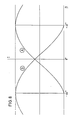
- the upper representation of FIG. 1 shows the frequency H of the detection signals of particles as a function of the axial position at which the particles cross the elongated focusing point.
- the axial length of a focal point is typically 0.4 mm.
- the centers of the focusing points F1 and F2 lie at the same distance fL (focal length) from the focusing device.
- the sensitivity characteristic is indicated by the cross-hatched areas in the beams. If the flow is at an angle to the normal to the optical axis OA of the focusing system in the plane of the rays S1 and S2 (the plane of the drawing), the frequency distributions are H a measurement can be selected two focus points that lie on a straight line that runs at a positive angle to the normal plane to the optical axis, while for the second measurement those focus points are selected that lie on a straight line that is at a negative angle to the aforementioned Normal plane runs.
- This method variant requires at least four focusing points, two of which lie on a common beam.
- the two beams can be generated by different polarization and subsequent spatial separation of light from the same light source.
- the amounts of the positive and negative angles of the straight lines passing through two pairs of focusing points are expediently the same with respect to the normal plane to the optical axis.
- FIG. 1 shows the measurement volume geometry of a two-dimensional two-focus method.
- the measuring volume MV of the flow channel two light beams S1 and S2, which run essentially parallel and at a short distance from one another, are focused at spatially separated focusing points F1 and F2.
- the axial extent L of the measurement volume MV is determined by the axial intensity distribution in the beams and by the beam path of the observing optics, which is optimized for the radiation centers.
- a particle that flies through the center of a focal point and is illuminated by the beam in question delivers a signal of maximum amplitude at a photodetector.
- the axial length L of the focusing point is chosen so that the same particle, when it flies through the edge region, only delivers a signal of one tenth of the maximum amplitude. Since in real currents the particles are always in size distributions (small particles provide a lower signal amplitude, but are more common than large particles), the small particles are still recognized in the axial center of the focal point, while only the much rarer large particles are recognized in the edge area.
- the upper representation of FIG. 1 shows the frequency H of the detection signals of particles as a function of the axial position at which the particles cross the elongated focusing point.
- the axial length of a focal point is typically 0.4 mm.
- the centers of the focusing points F1 and F2 are at the same distance fL (focal length) from the focusing device.
- the sensitivity characteristic is indicated by the cross-hatched areas in the beams. If the flow is at an angle to the normal to the optical axis OA of the focusing system in the plane of the rays S1 and S2 (the plane of the drawing), the frequency distributions are H the measured flight times t for different. Angle ⁇ shown in Fig. 3. If the angle ⁇ is not equal to zero, the effective axial length L of the measurement volume is reduced to L. This leads to a decrease in the frequency H with an increasing amount of the angle ⁇ . The influence of the flow angle ⁇ is increased by the above-mentioned axial sensitivity characteristic.
- the integral value I of the frequency distribution H is shown as a hatched area of the curves. This integral value 1 is, based on the measuring time, the measure for the measuring frequency.
- the dependence of the measuring rate on the flow angle ⁇ could be used to determine the axial component of the flow vector, but the measuring rate depends on many other parameters, such as e.g. Particle density. Laser power, sensitivity of the photodetectors u. Like. So that a clear calibration is practically not possible.
- FIG. 5 shows, in the same representation as FIG. 2, the case in which the focusing points F1 and F2 are axially offset from one another.
- the line connecting the centers of the focusing points F1 and F2 forms the angle y with the axis normal. If the angle ⁇ is changed by the focusing point F1 remaining fixed while the focusing point F2 is shifted axially parallel, the profile of the integral I shown in FIG. 6 (proportional to the measuring rate) is obtained as a function of the angle y. It can be seen that I assumes the maximum value when ⁇ is equal to ⁇ , that is to say when the straight line passing through the centers of the focusing points F1 and F2 runs exactly in the direction of flow. By determining the position of the maximum, the flow angle ⁇ can therefore be determined in relation to the normal to the optical axis of the system.
- the measurement method described assumes that the flow and measurement conditions remain unchanged during the shift of F2.
- the measuring rate then does not require any additional calibration.
- the maximum of the measuring rate will adjust to another value in a subsequent measuring cycle, the position of the maximum, i.e. the flow angle ⁇ , however, remains unchanged.
- a disadvantage is that the maximum of the curve shown in Fig. 6 runs very flat and therefore only allows an inaccurate position determination.
- the shifting of the focusing point F2 requires the acquisition of a series of measurements, which takes considerable time.
- the center of the focusing point F2 is offset by an angle y A of 45 ° from that of the focusing point F1.
- a particle which passes focus point F1 is recognized by a photodetector which generates a start signal, while a stop signal is generated when passing focus point F2 .
- FIG. 8 shows the integral I (or the measurement rate) over the angle ⁇ for both systems A and B according to FIG. 7.
- Fig. 9 is on (I B + I A) normalized difference (I B -I A) in terms of the size (I B -I A, provided (I B + I A). It can be seen that a good linearity of the curve results in. The flow angle ⁇ can thus be determined in a simple manner from the difference (I B -I A ).
- the curve can be determined by experimental calibration.
- the axial offset of the focusing points can be obtained in a simple manner by using a lens that is not completely chromatically corrected, so that different focal lengths result for different light colors.
- FIG. 10 shows a device with which the two measurements A and B can be carried out in succession.
- a tubular, elongated optical head OK is provided, into which an optical fiber cable LI leads.
- the light guide cable LI is a polarization-maintaining light guide cable, the decoupling unit LI o of which is arranged along the optical axis OA.
- the diverging multicolored light beam emerging from the decoupling unit Ll o is parallel by a lens L1 lized and fed along the optical axis of the focusing device FV.
- the focusing device FV contains a dispersion prism DP and a focusing lens LS1 in the beam path. The radiation emerges from the optical head OK behind the lens LS1 in order to be focused in the measurement volume MV.
- Radiation which is reflected by particles in the measurement volume MV, is directed in parallel by the lens LS1 and the parallel radiation is guided through the dispersion prism DP in the opposite direction to the incoming radiation and fed to the converging lens LS2, which focuses this radiation onto the coupling unit LII of a light guide LII .
- the collection lens has LS2 along the optical axis OA to a central opening through which passes the emerging from the coupling-unit Ll o beam.
- the dispersion prism DP demonstrates a spatial separation of the colors present in the incident light beam. These colors are focused in the measuring volume MV at focussing points which correspond to different deflection angles and are thus offset from one another transversely to the optical axis OA. In the present case, it is assumed that the green light component is focused at the focusing point F1, while the blue light component is focused at the focusing point F2. The other light components that are focused between the focusing points F1 and F2 can be disregarded for the described method.
- FIG. 10 a shows a top view of the device and FIG. 10 b) shows a side view of the device. It can be seen that the focusing points in the measurement volume MV are arranged in a plane containing the optical axis OA, but are laterally offset from one another in this plane.
- the centers of the focusing points F1 and F2 are also offset from one another in the direction of the optical axis OA, which is achieved in that the lens LS1 has chromatic properties, ie the individual light colors are focused with different focal lengths.
- the straight line passing through the centers of the focusing points F1 and F extends in the system A of FIG. 11 at an angle ⁇ A to the normal plane of the optical axis OA.
- the flow angle to the normal plane is designated ⁇ .
- the beam plane in which the axes of the beams SB and SG run, is rotated around the optical axis A by rotating the optical head OK such that the flow vector 1 lies in this plane.
- a relatively high measurement rate is obtained in measurement A in FIG. 11, since the angle ⁇ A characterizing the axial radiation offset is approximately equal to the flow angle. which the flow vector includes with the axis normal plane.
- the particles generate start pulses when they pass the focal point F1 of the green beam SG and stop pulses when they pass the focal point F2 of the blue beam SB.
- measurement B is carried out, in which the optical head OK is rotated around the optical axis OA with respect to measurement A by 180 °.
- the blue jet SB is now at the front in the direction of flow, so that the particles passing into the focusing point F2 produce start pulses, while stop pulses are generated when passing the focusing point F1 of the green beam.
- the angle ⁇ B which the straight line running through the centers of the focusing points F1 and F2 forms with the axis normal plane, is equal to the angle -y A.
- Measurement B gives only a very low measurement rate, since in this case the angle difference ⁇ -y e is very large.
- the flow angle ⁇ is obtained from the difference of the measuring rates in measurements A and B.
- the returning light reflected by particles in the measuring volume MV is directed in parallel by the lens LS1 and the different color components become reassembled in the dispersion prism DP.
- the returning light beam is fed into the light guide Lll by the collecting lens LS2.
- This light guide leads to a further dispersion prism DP2 outside the optical head.
- the green beam SG and the blue beam SB are spatially separated from one another and both beams are fed to the light receiving device LAV, which contains a photodetector PDG for the green light and a photodetector PDB for the blue light.
- the electrical signals of the two photodetectors are fed via a switchover unit UE to the evaluation unit AE, which contains a start signal generator and a stop signal generator.
- the switchover unit UE establishes the connections shown in solid lines in FIG. 10, the output of the photodetector PDG generating the start signals, while the output of the photodetector PDB generating the stop signals.
- the switchover unit UE produces the connections shown in broken lines, the photodetector PDB generating the start signals and the photodetector PDG generating the stop signals.
- FIGS. 12 and 13 An exemplary embodiment is shown in FIGS. 12 and 13, in which measurements A and B can be carried out simultaneously.
- the optical head OK is designed in the same way as that of FIG. 10, but a polarization prism PP1 is provided instead of the dispersion prism.
- a further polarization prism PP2 is arranged between the lens LS2 and the polarization prism PP1, which has a central opening for the passage of the incoming beam.
- the light guide LI is a single-mode light guide with polarization-maintaining properties.
- the multicolored light supplied to this light guide LI is linearly polarized at 45 °.
- the polarization prism PP1 the incoming light is divided into two beams of equal intensity, polarized perpendicular to each other, which have different exit angles and are thus spatially separated from one another.
- the lens LS1 thus gives two focused beams S1 and S2 in the measurement volume MV with different directions of polarization. Since both beams are multi-colored, the individual colors of both beams are imaged on their smallest diameter at different axial locations with a suitable chromatic focal length distribution of the lens LS1. This is shown in Fig. 13.
- the green components of the two beams S1 and S2 have green focusing points FG1 and FG2 at the same axial distance from the focusing device FV and the blue focusing points FB1 and FB2 are also at the same distance from each other from the focusing device FV, but this distance is the blue focusing points from the focusing device larger than that of the green focus points from the focusing device.
- Beam S1 is polarized in parallel and beam S2 is polarized perpendicularly.
- the focus point FG1 is used to generate the start pulses and the focus point FB2 is used to generate the stop pulses.
- the straight line passing through the centers of these focusing points forms the angle y A with the normal plane to the optical axis OA.
- the focus point FB1 is used to generate the start pulses and the focus point FG2 is used to generate the stop pulses.
- the straight line passing through the centers of these two focusing points forms with the normal plane to the optical axis OA the angle ⁇ B which is -y A.
- the scattered light from the measurement volume MV is collected by the outer area of the lens LS1 and passed through the polarization beam splitter PP1. whereby the color offset and the division in the two polarization directions is reversed again.
- the further polarization beam splitter PP2 which is provided with a central opening, is used to image the differently polarized scattered light from the focusing points onto two coupling units LI11, and L112 1 that are sufficiently separated by means of the lens LS2.
- the light guides LII1 and L112 connected to the coupling units each lead to a color division unit FA1 or FA2, which spatially separates the components of interest blue and green from the multicolored light.
- the color splitting unit FA1 receives the parallel polarized light component and the color splitting unit FA2 the perpendicularly polarized light component.
- the color splitting unit FA1 generates a parallel polarized blue beam BP and a parallel polarized green beam GP. These beams are converted into electrical signals by the PDBP and PDGB photodetectors.
- the color splitting unit FA2 generates a blue beam BV and a green beam GV from the perpendicularly polarized beam, which are spatially separated from one another and are each supplied to the photodetectors PDBV and PDGV, which generate electrical pulses depending on the intensities of these light beams.
- the output signal of the photodetector PDGB is fed to the evaluation unit AE A for measurement A and generates a start pulse there, while the output signal of the photodetector PDBV generates a stop pulse in the evaluation unit AE A.
- the output signal of the photodetector PDBP is fed to the evaluation unit AE B for the second measurement B and generates a start pulse there, while the output signal of the photodetector PDBV is also fed to the evaluation unit AE B and generates a stop pulse there.
- Both measuring systems A and B register the same speed of the vector v.
- the evaluation electronics therefore only need to be carried out for one system. Only the measuring rate must be simultaneous for both systems A and B. and be determined independently of each other. This requires a relatively small additional electronic effort.
- FIG. 14 Another, even simpler variant of the method is shown in FIG. 14.
- the beam path shown in FIG. 13 is also generated in the measurement volume MV.
- the optical head OK of the device of FIG. 14 differs from that of FIG. 12 only in that the polarization beam splitter PP2 is omitted and in that the lens LS2 focuses the returning radiation onto a single coupling element LII, to which the single color splitting unit FA leading light guide Lil is connected.
- the color splitting unit FA selects the green component G and the blue component B from the returning light beam, which are individually fed to the light receiving device LAV, which contains a photodetector PDG for the green light beam and a photodetector PDB for the blue light beam.
- the output signal of the photodetector PDG is fed to the evaluation unit AE A for measurement A as a start signal, while the output signal of the photodetector PDB for the blue light is fed to the evaluation unit AE A as a stop signal.
- the evaluation unit AE B for the second measurement B receives the output signal of the photodetector PDB as the start signal and the output signal of the photodetector PDG as the stop signal.
- the different polarization of the two beams S1 and S2 is only used to spatially separate these beams from one another.
- the evaluation of the different light components takes place without considering the polarization direction exclusively on the basis of the color components.
- Both photodetectors PDG and PDB register the entire scattered light from the measurement volume. Although the scattered light which is generated by the beams S1 and S2 is polarized differently, after the scattered light has been passed on through the light guide LII, it is no longer possible to separate it into two mutually perpendicularly polarized scattered light components.
- a single photodetector e.g. with PDG, a speed measurement possible.
- the direction of the speed (whether from beam S1 to beam S2 or vice versa) can no longer be recognized. This is not a disadvantage in a large number of applications, since the approximate flow direction is usually known beforehand.
- the same speed would be measured with the PDB photodetector as with the PDG photodetector. It is assumed that the speed in the measurement volume does not change over the length of the axial measurement location offset of the two colors, which is typically about 0.2 mm.
- the information from both evaluation units is passed on to a multi-channel analyzer which displays the time measurements between start pulses and stop pulses as a frequency distribution.
- the integral I or the area under the frequency curve, is a measure of the measuring rate.
- the position of the measurement curve indicates the size of the two-dimensional speed vector v in the normal plane to the optical axis OA.
- the direction of the vector in the normal plane is determined beforehand in each case by rotating the optical head OK around the optical axis OA until the frequency distribution assumes a maximum. In this angular position of the optical head, the vector component running in the direction of the optical axis is then measured.
Abstract
Bei der optischen Messung der Strömungsvektoren in Gasströmungen werden zwei im wesentlichen parallele Lichtstrahlen an getrennten Fokussierungsstellen fokussiert. Die die eine Fokussierungsstelle passierenden Teilchen leuchten auf und erzeugen dadurch Startimpulse. Die die andere Fokussierungsstelle passierenden Teilchen erzeugen beim Aufleuchten Stopimpulse. Mit solchen Verfahren kann die in der Normalenebene zur optischen Achse (OA) verlaufende Komponente des Strömungsvektors (v) ermittelt werden. Der Erfindung liegt die Aufgabe zugrunde, mit einfachen Mitteln auch die parallel zur optischen Achse (OA) verlaufende Komponente des Strömungsvektors zu erfassen. Nach der Erfindung werden Fokussierungsstellen (FG1, FB2; FB1, FG2) der Strahlen (S1, S2) mit unterschiedlichen Brennweiten erzeugt. In einer ersten Messung (A) wird die durch die Fokussierungsstellen (FG1) und (FB2) durchgehende Gerade unter einem Winkel (γA) zur Normalenebene der optischen Achse gebildet und bei einer zweiten Messung (B) wird die durch die Fokussierungsstellen (FB1, FG2) hindurchgehende Gerade unter einem Winkel (γB = -γA) erzeugt, der das entgegengesetzte Vorzeichen zum ersten Winkel hat. Durch Differenzbildung der beiden Meßraten wird der Strömungswinkel (β) in Bezug auf die Normalenebene zur optischen Achse (OA) ermittelt.In the optical measurement of the flow vectors in gas flows, two substantially parallel light beams are focused at separate focusing points. The particles that pass through a focal point light up and thereby generate start impulses. The particles passing the other focal point generate stop pulses when illuminated. With such methods, the component of the flow vector (v) running in the normal plane to the optical axis (OA) can be determined. The invention is based on the object of also using simple means to detect the component of the flow vector running parallel to the optical axis (OA). According to the invention, focusing points (FG1, FB2; FB1, FG2) of the beams (S1, S2) are generated with different focal lengths. In a first measurement (A) the straight line passing through the focusing points (FG1) and (FB2) is formed at an angle (γA) to the normal plane of the optical axis and in a second measurement (B) the straight line through the focusing points (FB1, FG2 ) straight line generated at an angle (γB = -γA) that has the opposite sign to the first angle. The flow angle (β) in relation to the normal plane to the optical axis (OA) is determined by forming the difference between the two measuring rates.
Description
Die Erfindung betrifft ein Verfahren nach dem Oberbegriff des Patentanspruchs 1 sowie eine Vorrichtung zur Durchführung des Verfahrens.The invention relates to a method according to the preamble of
Zur Messung von Strömungsvektoren in Gasströmungen ist es bekannt, das Licht einer Lichtquelle mit einer Fokussiervorrichtung in dem Strömungskanal an zwei dicht hintereinander angeordneten Fokussierungsstellen zu fokussieren (DE-PS 24 49 358). Die in der Gasströmung enthaltenen Teilchen werden, wenn sie die Fokussierungsstellen passieren, beleuchtet. Die von den Teilchen reflektierte Streustrahlung erzeugt beim Passieren der ersten Fokussierungsstelle einen Startimpuls und beim Passieren der zweiten Fokussierungsstelle einen Stopimpuls. Aus dem zeitlichen Abstand von Startimpuls und Stopimpuls kann die Komponente des Vektors der Teilchenge-![]()
![]()
Es zeigen:
- Fig. 1 eine Ansicht der Geometrie des Meßvolumens bei zwei Fokussierungsstellen, die den gleichen Abstand von der Fokussiervorrichtung haben, wobei die Häufigkeitsverteilung der Erkennung von Teilchendurchgängen als Funktion der axialen Position, bei der die Teilchen die Strahlen durchqueren, dargestellt ist,
- Fig. 2 eine Darstellung zweier Fokussierungsstellen mit eingezeichneter Empfindlichkeitscharakteristik,
- Fig. 3 zwei graphische Darstellungen der Häufigkeit von Meßergebnissen bei unterschiedlichen Winkeln β der Strömung in Bezug auf die Normalenebene zur optischen Achse,
- Fig. 4 eine Darstellung des Integralwertes I der Häufigkeitsverteilung über dem Winkel ß,
- Fig. 5 eine Darstellung der Verhaltnisse bei in Richtung der optischen Achse gegeneinander versetzten Fokussierungsstellen,
- Fig. 6 die in Fig. 4 dargestellte Häufigkeitsverteilung bei der Anordnung der Fokussierungsstellen gemäß Fig. 5,
- Fig. 7 eine Darstellung zweier Systeme A und B unterschiedlich gegeneinander versetzter Fokussierungsstellen,
- Fig. 8 die Integralwerte der Häufigkeitsverteilungen (Meßraten) bei den beiden Systemen nach Fig. 7 über dem Winkel ß,
- Fig. 9 eine graphische Darstellung der normierten Differenz der Meßraten über dem Strömungswinkel β zur Verdeutlichung der Linearität zwischen der Differenz und dem Winkel β,
- Fig. 10 eine Draufsicht und eine Seitenansicht einer ersten Ausführungsform der Meßvorrichtung,
- 1 is a view of the geometry of the measuring volume at two focusing points that are at the same distance from the focusing device, the frequency distribution of the detection of particle passages being shown as a function of the axial position at which the particles cross the beams,
- 2 shows a representation of two focussing points with the sensitivity characteristic shown,
- 3 shows two graphical representations of the frequency of measurement results at different angles β of the flow in relation to the normal plane to the optical axis,
- 4 shows a representation of the integral value I of the frequency distribution over the angle β,
- 5 shows a representation of the conditions in the case of focusing points offset in the direction of the optical axis,
- 6 shows the frequency distribution shown in FIG. 4 in the arrangement of the focusing points according to FIG. 5,
- 7 shows a representation of two systems A and B differently offset focusing points,
- 8 shows the integral values of the frequency distributions (measuring rates) in the two systems according to FIG. 7 over the angle β,
- 9 is a graphical representation of the normalized difference of the measuring rates over the flow angle β to clarify the linearity between the difference and the angle β,
- 10 is a plan view and a side view of a first embodiment of the measuring device,
tein erfaßt werden kann, so daß der Strömungsvektor im dreidimensionalen Raum unter Verwendung von nur zwei Lichtstrahlen erfaßt werden kann.tein can be detected so that the flow vector can be detected in three-dimensional space using only two light beams.
Die Lösung dieser Aufgabe erfolgt erfindunggemäß mit den im kennzeichnenden Teil des Patentanspruchs 1 angegebenen Merkmalen.This object is achieved according to the invention with the features specified in the characterizing part of
Nach der Erfindung werden die Fokussierungsstellen, die unterschiedliche Abstände von der optischen Achse haben, zusätzlich auch in Richtung der optischen Achse gegeneinander versetzt. Dabei wird eine erste Messung durchgeführt, bei der die Fokussiervorrichtung des einen Strahls näher an der Fokussierungsstelle liegt als diejenige des anderen Strahls und bei einer zweiten Messung werden diese Verhältnisse umgekehrt, so daß die Fokussierungsstelle des ersten Strahls weiter von der Fokussiervorrichtung entfernt ist als diejenige Fokussierungsstellen F1 und F2 fokussiert. Die axiale Erstreckung L des Meßvolumens MV wird bestimmt durch die axiale Intensitätsverteilung in den Strahlen und durch den Strahlengang der beobachtenden Optik, der auf die Strahlenzentren optimiert ist. Ein Teilchen, das durch das Zentrum einer Fokussierungsstelle fliegt und durch den betreffenden Strahl beleuchtet wird, liefert an einem Photodetektor ein Signal maximaler Amplitude. Die axiale Länge L der Fokussierungsstelle ist so gewählt, daß dasselbe Teilchen, wenn es durch den Randbereich fliegt, nur ein Signal von einem Zehntel der maximalen Amplitude liefert. Da in realen Strömungen die Teilchen immer in Größenverteilungen vorliegen (kleine Teilchen liefern eine geringere Signalamplitude, sind allerdings häufiger als große Teilchen), werden im axialen Zentrum der Fokussierungsstelle die kleinen Teilchen noch erkannt, während im Randbereich nur die viel selteneren großen Teilchen erkannt werden. In der oberen Darstellung von Fig. 1 ist die Häufigkeit H der Erkennungssignale von Teilchen als Funktion der axialen Position, bei der die Teilchen die langgestreckte Fokussierungsstelle durchqueren, dargestellt. Die axiale Länge einer Fokussierungsstelle beträgt typischerweise 0,4 mm.According to the invention, the focusing points, which have different distances from the optical axis, are also offset from one another in the direction of the optical axis. A first measurement is carried out in which the focusing device of one beam is closer to the focusing point than that of the other beam and a second measurement reverses these conditions, so that the focusing point of the first beam is further away from the focusing device than that focusing point F1 and F2 focused. The axial extent L of the measurement volume MV is determined by the axial intensity distribution in the beams and by the beam path of the observing optics, which is optimized for the radiation centers. A particle that flies through the center of a focal point and is illuminated by the beam in question delivers a signal of maximum amplitude at a photodetector. The axial length L of the focusing point is chosen so that the same particle, when it flies through the edge region, only delivers a signal of one tenth of the maximum amplitude. Since in real currents the particles are always in size distributions (small particles provide a lower signal amplitude, but are more common than large particles), the small particles are still recognized in the axial center of the focal point, while only the much rarer large particles are recognized in the edge area. The upper representation of FIG. 1 shows the frequency H of the detection signals of particles as a function of the axial position at which the particles cross the elongated focusing point. The axial length of a focal point is typically 0.4 mm.
Bei dem in Fig. 2 dargestellten Strahlenpaar S1, S2 liegen die Zentren der Fokussierungsstellen F1 und F2 in demselben AbstandfL (Brennweite) von der Fokussiervorrichtung. Die Empfindlichkeitscharakteristik ist durch die kreuzschraffierten Flächen in den Strahlen angedeutet. Wenn die Strömung unter einem Winkel zur Normalen zur optischen Achse OA des Fokussierungssystems in der Ebene der Strahlen S1 und S2 (der Zeichnungsebene) verläuft, sind die Häufigkeitsverteilungen H eine Messung können zwei Fokussierungsstellen ausgewählt werden, die auf einer Geraden liegen, welche unter positivem Winkel zu der Normalenebene zur optischen Achse verläuft, während für die zweite Messung solche Fokussierungsstellen ausgewählt werden, die auf einer Geraden liegen, welche unter einem negativen Winkel zu der genannten Normalenebene verläuft. Für diese Verfahrensvariante benötigt man mindestens vier Fokussierungsstellen, von denen jeweils zwei auf einem gemeinsamen Strahl liegen. Die beiden Strahlen können durch unterschiedliche Polarisierung und anschließende räumliche Trennung von Licht derselben Lichtquelle erzeugt werden. Zweckmäßigerweise sind die Beträge des positiven und des negativen Winkels der durch zwei Paare von Fokussierungsstellen hindurchgehenden Geraden in Bezug auf die Normalenebene zur optischen Achse einander gleich.In the case of the beam pair S1, S2 shown in FIG. 2, the centers of the focusing points F1 and F2 lie at the same distance fL (focal length) from the focusing device. The sensitivity characteristic is indicated by the cross-hatched areas in the beams. If the flow is at an angle to the normal to the optical axis OA of the focusing system in the plane of the rays S1 and S2 (the plane of the drawing), the frequency distributions are H a measurement can be selected two focus points that lie on a straight line that runs at a positive angle to the normal plane to the optical axis, while for the second measurement those focus points are selected that lie on a straight line that is at a negative angle to the aforementioned Normal plane runs. This method variant requires at least four focusing points, two of which lie on a common beam. The two beams can be generated by different polarization and subsequent spatial separation of light from the same light source. The amounts of the positive and negative angles of the straight lines passing through two pairs of focusing points are expediently the same with respect to the normal plane to the optical axis.
Im folgenden werden unter Bezugnahme auf die Zeichnungen Ausführungsbeispiele der Erfindung näher erläutert.Exemplary embodiments of the invention are explained in more detail below with reference to the drawings.
Es zeigen:Show it:
- Fig. 1 eine Ansicht der Geometrie des Meßvolumens bei zwei Fokussierungsstellen, die den gleichen Abstand von der Fokussiervorrichtung haben, wobei die Häufigkeitsverteilung der Erkennung von Teilchendurchgängen als Funktion der axialen Position, bei der die Teilchen die Strahlen durchqueren, dargestellt ist,1 is a view of the geometry of the measuring volume at two focusing points which are at the same distance from the focusing device, the frequency distribution of the detection of particle passages being shown as a function of the axial position at which the particles cross the beams,
- Fig. 2 eine Darstellung zweier Fokussierungsstellen mit eingezeichneter Empfindlichkeitscharakteristik.2 shows a representation of two focussing points with the sensitivity characteristic shown.
- Fig. 3 zwei graphische Darstellungen der Häufigkeit von Meßergebnissen bei unterschiedlichen Winkeln β der Strömung in Bezug auf die Normalenebene zur optischen Achse,3 shows two graphical representations of the frequency of measurement results at different angles β of the flow in relation to the normal plane to the optical axis,
- Fig. 4 eine Darstellung des Integralwertes I der Häufigkeitsverteilung über dem Winkel ß,4 shows a representation of the integral value I of the frequency distribution over the angle β,
- Fig. 5 eine Darstellung der Verhaltnisse bei in Richtung der optischen Achse gegeneinander versetzten Fokussierungsstellen,5 shows a representation of the conditions in the case of focussing points offset in the direction of the optical axis,
- Fig. 6 die in Fig. 4 dargestellte Häufigkeitsverteilung bei der Anordnung der Fokussierungsstellen gemäß Fig. 5,6 shows the frequency distribution shown in FIG. 4 in the arrangement of the focusing points according to FIG. 5,
- Fig. 7 eine Darstellung zweier Systeme A und B unterschiedlich gegeneinander versetzter Fokussierungsstellen,7 shows a representation of two systems A and B differently offset focusing points,
- Fig. 8 die Integralwerte der Häufigkeitsverteilungen (Meßraten) bei den beiden Systemen nach Fig. 7 über dem Winkel ß,8 shows the integral values of the frequency distributions (measuring rates) in the two systems according to FIG. 7 over the angle β,
- Fig. 9 eine graphische Darstellung der normierten Differenz der Meßraten über dem Strömungswinkel β zur Verdeutlichung der Linearität zwischen der Differenz und dem Winkel β,9 is a graphical representation of the normalized difference of the measuring rates over the flow angle β to clarify the linearity between the difference and the angle β,
- Fig. 10 eine Draufsicht und eine Seitenansicht einer ersten Ausführungsform der Meßvorrichtung,10 is a plan view and a side view of a first embodiment of the measuring device,
- Fig. 11 die unterschiedliche Anordnung der Fokussierungsstellen bei der Vorrichtung nach Fig. 10. wenn die Fokussiervorrichtung um 180° gedreht wird, um von dem Meßsystem A auf das Meßsystem B überzugehen,11 shows the different arrangement of the focusing points in the device according to FIG. 10 when the focusing device is rotated by 180 ° in order to pass from the measuring system A to the measuring system B,
- Fig. 12 eine Draufsicht und eine Seitenansicht einer zweiten Ausführungsform der Meßvorrichtung,12 is a plan view and a side view of a second embodiment of the measuring device,
- Fig. 13 eine Darstellung der vier Fokussierungs stellen, die sich bei der Vorrichtung nach Fig. 12 ergeben undFig. 13 is an illustration of the four focus, which result in the device of FIG. 12 and
- Fig. 14 eine gegenüber Fig. 12 vereinfachte weitere Ausführungsform der Vorrichtung.FIG. 14 shows a further embodiment of the device which is simplified compared to FIG. 12.
Zunächst werden unter Bezugnahme auf die Fign. 1 bis 9 die Grundlagen erläutert, die für das Verständnis der Erfindung erforderlich sind.First, with reference to Figs. 1 to 9 explain the basics required for understanding the invention.
In Fig. 1 ist die Meßvolumengeometrie eines zweidimensionalen Zwei-Fokus-Verfahrens dargestellt. Im Meßvolumen MV des Strömungskanals werden zwei Lichtstrahlen S1 und S2, die im wesentlichen parallel und mit geringem Abstand zueinander verlaufen, an räumlich getrennten Fokussierungsstellen F1 und F2 fokussiert. Die axiale Erstreckung L des Meßvolumens MV wird bestimmt durch die axiale Intensitätsverteilung in den Strahlen und durch den Strahlengang der beobachtenden Optik, der auf die Strahlenzentren optimiert ist. Ein Teilchen, das durch das Zentrum einer Fokussierungsstelle fliegt und durch den betreffenden Strahl beleuchtet wird, liefert an einem Photodetektor ein Signal maximaler Amplitude. Die axiale Länge L der Fokussierungsstelle ist so gewählt, daß dasselbe Teilchen, wenn es durch den Randbereich fliegt, nur ein Signal von einem Zehntel der maximalen Amplitude liefert. Da in realen Strömungen die Teilchen immer in Größenverteilungen vorliegen (kleine Teilchen liefern eine geringere Signalamplitude, sind allerdings häufiger als große Teilchen), werden im axialen Zentrum der Fokussierungsstelle die kleinen Teilchen noch erkannt, während im Randbereich nur die viel selteneren großen Teilchen erkannt werden. In der oberen Darstellung von Fig. 1 ist die Häufigkeit H der Erkennungssignale von Teilchen als Funktion der axialen Position, bei der die Teilchen die langgestreckte Fokussierungsstelle durchqueren, dargestellt. Die axiale Länge einer Fokussierungsstelle beträgt typischerweise 0,4 mm.1 shows the measurement volume geometry of a two-dimensional two-focus method. In the measuring volume MV of the flow channel, two light beams S1 and S2, which run essentially parallel and at a short distance from one another, are focused at spatially separated focusing points F1 and F2. The axial extent L of the measurement volume MV is determined by the axial intensity distribution in the beams and by the beam path of the observing optics, which is optimized for the radiation centers. A particle that flies through the center of a focal point and is illuminated by the beam in question delivers a signal of maximum amplitude at a photodetector. The axial length L of the focusing point is chosen so that the same particle, when it flies through the edge region, only delivers a signal of one tenth of the maximum amplitude. Since in real currents the particles are always in size distributions (small particles provide a lower signal amplitude, but are more common than large particles), the small particles are still recognized in the axial center of the focal point, while only the much rarer large particles are recognized in the edge area. The upper representation of FIG. 1 shows the frequency H of the detection signals of particles as a function of the axial position at which the particles cross the elongated focusing point. The axial length of a focal point is typically 0.4 mm.
Bei dem in Fig. 2 dargestellten Strahlenpaar S1, S2 liegen die Zentren der Fokussierungsstellen F1 und F2 in demselben AbstandfL (Brennweite) von der Fokussiervorrichtung. Die Empfindlichkeitscharakteristik ist durch die kreuzschraffierten Flächen in den Strahlen angedeutet. Wenn die Strömung unter einem Winkel zur Normalen zur optischen Achse OA des Fokussierungssystems in der Ebene der Strahlen S1 und S2 (der Zeichnungsebene) verläuft, sind die Häufigkeitsverteilungen H der gemessenen Flugzeiten t für verschiedene. Winkel β in Fig. 3 dargestellt. Wenn der Winkel β ungleich Null ist, verkürzt sich die wirksame axiale Länge L des Meßvolumens auf L. Dies führt zur Abnahme der Häufigkeit H mit zunehmendem Betrag des Winkels β. Der Einfluß des Strömungswinkels β wird durch die oben erwähnte axiale Empfindlichkeitscharakteristik verstärkt.In the case of the beam pair S1, S2 shown in FIG. 2, the centers of the focusing points F1 and F2 are at the same distance fL (focal length) from the focusing device. The sensitivity characteristic is indicated by the cross-hatched areas in the beams. If the flow is at an angle to the normal to the optical axis OA of the focusing system in the plane of the rays S1 and S2 (the plane of the drawing), the frequency distributions are H the measured flight times t for different. Angle β shown in Fig. 3. If the angle β is not equal to zero, the effective axial length L of the measurement volume is reduced to L. This leads to a decrease in the frequency H with an increasing amount of the angle β. The influence of the flow angle β is increased by the above-mentioned axial sensitivity characteristic.
In Fig. 3 ist der Integralwert I der Häufigkeitsverteilung H jeweils als schraffierter Bereich der Kurven dargestellt. Dieser Integralwert 1 ist, bezogen auf die Meßzeit, das Maß für die Meßfrequenz.In Fig. 3, the integral value I of the frequency distribution H is shown as a hatched area of the curves. This
In Fig. 4 ist der Integralwert I (proportional zur Häufigkeit von Meßergebnissen = Meßrate) über dem Strömungswinkel β aufgetragen. Man könnte die Abhängigkeit der Meßrate vom Strömungswinkel β zur Bestimmung der Axialkomponente des Strömungsvektors nutzen, jedoch ist die Meßrate von vielen anderen Parametern abhängig, wie z.B. Teilchendichte. Laserleistung, Empfindlichkeit der Photodetektoren u. dgl., so daß eine eindeutige Kalibrierung praktisch nicht möglich ist.4, the integral value I (proportional to the frequency of measurement results = measurement rate) is plotted against the flow angle β. The dependence of the measuring rate on the flow angle β could be used to determine the axial component of the flow vector, but the measuring rate depends on many other parameters, such as e.g. Particle density. Laser power, sensitivity of the photodetectors u. Like. So that a clear calibration is practically not possible.
Fig. 5 zeigt in gleicher Darstellung wie Fig. 2 den Fall, daß die Fokussierungsstellen F1 und F2 axial gegeneinander versetzt sind. Die Verbindungslinie der Zentren der Fokussierungsstellen F1 und F2 bildet mit der Achsennormalen den Winkel y . Verändert man den Winkel γ,indem die Fokussierungsstelle F1 fest bleibt, während die Fokussierungsstelle F2 achsparallel verschoben wird, so ergibt sich der in Fig. 6 dargestellte Verlauf des Integrals I (proportional zur Meßrate) in Abhängigkeit vom Winkel y . Man erkennt, daß I den Maximalwert annimmt, wenn γ gleich β ist, also wenn die durch die Zentren der Fokussierungsstellen F1 und F2 hindurchgehende Gerade genau in Strömungsrichtung verläuft. Durch Ermittlung der Lage des Maximums kann daher der Strömungswinkel β in Bezug auf die Normale zur optischen Achse des Systems festgestellt werden.5 shows, in the same representation as FIG. 2, the case in which the focusing points F1 and F2 are axially offset from one another. The line connecting the centers of the focusing points F1 and F2 forms the angle y with the axis normal. If the angle γ is changed by the focusing point F1 remaining fixed while the focusing point F2 is shifted axially parallel, the profile of the integral I shown in FIG. 6 (proportional to the measuring rate) is obtained as a function of the angle y. It can be seen that I assumes the maximum value when γ is equal to β, that is to say when the straight line passing through the centers of the focusing points F1 and F2 runs exactly in the direction of flow. By determining the position of the maximum, the flow angle β can therefore be determined in relation to the normal to the optical axis of the system.
Das beschriebene Meßverfahren setzt voraus, daß während der Verschiebung von F2 die Strömungs-und Meßverhältnisse unverändert bleiben. Die Meßrate bedarf dann keiner zusätzlichen Kalibrierung. Bei Veränderung der oben erwähnten Parameter, wie z.B. der Laserleistung, wird sich bei einem nachfolgenden Meßzyklus zwar das Maximum der Meßrate auf einen anderen Wert einstellen, die Lage des Maximums, d.h. der Strömungswinkel β, bleibt jedoch unverändert. Nachteilig ist, daß das Maximum der in Fig. 6 dargestellten Kurve sehr flach verläuft und daher nur eine ungenaue Lage bestimmung ermöglicht. Ferner erfordert die Verschiebung der Fokussierungsstelle F2 die Aufnahme einer Meßreihe, wozu erhebliche Zeit benötigt wird.The measurement method described assumes that the flow and measurement conditions remain unchanged during the shift of F2. The measuring rate then does not require any additional calibration. When changing the parameters mentioned above, e.g. the laser power, the maximum of the measuring rate will adjust to another value in a subsequent measuring cycle, the position of the maximum, i.e. the flow angle β, however, remains unchanged. A disadvantage is that the maximum of the curve shown in Fig. 6 runs very flat and therefore only allows an inaccurate position determination. Furthermore, the shifting of the focusing point F2 requires the acquisition of a series of measurements, which takes considerable time.
Das erfindungsgemäße Verfahren wird nun in seinen Grundzügen anhand von Fig. 7 erläutert.The principles of the method according to the invention will now be explained with reference to FIG. 7.
Bei dem System A ist das Zentrum der Fokussierungsstelle F2 gegenüber demjenigen der Fokussierungsstelle F1 um den Winkel yA 45° versetzt.In system A, the center of the focusing point F2 is offset by an angle y A of 45 ° from that of the focusing point F1.
Bei dem darunter dargestellten System ist dagegen die Fokussierungsstelle F2 gegenüber F1 um den Winkel γB = -45° versetzt. System A weist bei Strömungsvektoren mit β = +45° die größte Signalrate auf, während bei Strömungswinkeln von β = -45° die Meßrate auf Null zurückgeht. Dasselbe gilt umgekehrt für System B. In Fig. 7 ist ferner eingezeichnet, daß ein Teilchen, das die Fokussierungsstelle F1 passiert, von einem Photodetektor erkannt wird, der ein Start-Signal erzeugt, während beim Passieren der Fokussierungsstelle F2 ein Stop-Signal erzeugt wird.In contrast, in the system shown below, the focusing point F2 is offset by an angle γ B = -45 ° with respect to F1. System A has the highest signal rate for flow vectors with β = +4 5 ° , while the measurement rate drops to zero for flow angles of β = -45 °. The same applies vice versa for system B. It is also shown in FIG. 7 that a particle which passes focus point F1 is recognized by a photodetector which generates a start signal, while a stop signal is generated when passing focus point F2 .
Fig. 8 zeigt das Integral I (bzw. die Meßrate) über dem Winkel β für beide Systeme A und B nach Fig. 7. Für Strömungswinket β = 0°, weisen beide Systeme eine Meßrate von etwa 60% der maximalen Meßrate auf. Man erkennt, daß beide Systeme für Strömungswinkel im Bereich von -30° < β < + 30° eine nahezu lineare Charakteristik und eine hohe Empfindlichkeit aufweisen. Wenn man nun mit beiden Systemen an demselben Meßort mißt, kann man aus dem Unterschied der Meßraten der Systeme A und B den Strömungswinkel β ermitteln.FIG. 8 shows the integral I (or the measurement rate) over the angle β for both systems A and B according to FIG. 7. For flow angles β = 0 °, both systems have a measurement rate of approximately 60% of the maximum measurement rate. It can be seen that both systems have a nearly linear characteristic and a high sensitivity for flow angles in the range from -30 ° <β <+ 30 °. If you now measure with both systems at the same measuring location, you can determine the flow angle β from the difference in the measuring rates of systems A and B.
In Fig. 9 ist die auf (IB + IA) normierte Differenz (IB -IA) in Form der Größe (IB -IA,(IB + IA) dar gestellt. Man erkennt, daß sich eine gute Linearität der Kurve ergibt. Aus der Differenz (IB -IA) kann somit auf einfache Weise der Strömungswinkel ß ermittelt werden.In Fig. 9 is on (I B + I A) normalized difference (I B -I A) in terms of the size (I B -I A, provided (I B + I A). It can be seen that a good linearity of the curve results in. The flow angle β can thus be determined in a simple manner from the difference (I B -I A ).
Die in Fig. 9 dargestellte Beziehung ist im wesentlichen nur noch abhängig vom Achsversatz der Fokussierungsstellen, der durch die Winkel γA und γB (in diesem Beispiel ist yA = +45°und γB = -45°) gekennzeichnet werden kann, und von der axialen Erstreckung L der Fokussierungsstellen.The relationship shown in FIG. 9 is essentially only dependent on the axis offset of the focusing points, which can be characterized by the angles γ A and γ B (in this example, y A = + 45 ° and γ B = -45 °), and the axial extent L of the focusing points.
Die Kurve kann durch experimentelle Eichung ermittelt werden.The curve can be determined by experimental calibration.
Der axiale Versatz der Fokussierungsstellen kann auf einfache Weise dadurch erhalten werden, daß man eine Linse verwendet, die nicht vollständig chromatisch korrigiert ist, so daß sich für verschiedene Lichtfarben unterschiedliche Brennweiten ergeben.The axial offset of the focusing points can be obtained in a simple manner by using a lens that is not completely chromatically corrected, so that different focal lengths result for different light colors.
In Fig. 10 ist eine Vorrichtung dargestellt, mit der die beiden Messungen A und B nacheinander durchgeführt werden können.10 shows a device with which the two measurements A and B can be carried out in succession.
Gemäß Fig. 10 ist ein rohrförmiger langgestreckter optischer Kopf OK vorgesehen, in den ein Lichtleiterkabel LI hineinführt. Das Lichtleiterkabel LI ist ein polarisationserhaltendes Lichtleiterkabel, dessen Auskopplungseinheit LIo längs der optischen Achse OA angeordnet ist. Der divergierend aus der Auskopplungseinheit Llo austretende mehrfarbige Lichtstrahl wird durch eine Linse L1 parallelisiert und entlang der optischen Achse der Fokussiervorrichtung FV zugeführt. Die Fokussiervorrichtung FV enthält hintereinander im Strahlengang ein Dispersionsprisma DP und eine Fokussierungslinse LS1. Hinter der Linse LS1 tritt die Strahlung aus dem optischen Kopf OK aus, um in dem Meßvolumen MV fokussiert zu werden.10, a tubular, elongated optical head OK is provided, into which an optical fiber cable LI leads. The light guide cable LI is a polarization-maintaining light guide cable, the decoupling unit LI o of which is arranged along the optical axis OA. The diverging multicolored light beam emerging from the decoupling unit Ll o is parallel by a lens L1 lized and fed along the optical axis of the focusing device FV. The focusing device FV contains a dispersion prism DP and a focusing lens LS1 in the beam path. The radiation emerges from the optical head OK behind the lens LS1 in order to be focused in the measurement volume MV.
Strahlung, die von Teilchen im Meßvolumen MV reflektiert wird, wird von der Linse LS1 parallel gerichtet und die parallele Strahlung wird durch das Dispersionsprisma DP in Gegenrichtung zur hinlaufenden Strahlung geleitet und der Sammellinse LS2 zugeführt, die diese Strahlung auf die Einkoppeleinheit LII eines Lichtleiters LII fokussiert.Radiation, which is reflected by particles in the measurement volume MV, is directed in parallel by the lens LS1 and the parallel radiation is guided through the dispersion prism DP in the opposite direction to the incoming radiation and fed to the converging lens LS2, which focuses this radiation onto the coupling unit LII of a light guide LII .
Die Sammellinse LS2 weist entlang der optischen Achse OA eine Mittelöffnung auf, durch die der aus der Auskopplungseinheit Llo austretende Strahl hindurchgeht.The collection lens has LS2 along the optical axis OA to a central opening through which passes the emerging from the coupling-unit Ll o beam.
Das Dispersionsprisma DP führt eine räumliche Trennung der im einfallenden Lichtstrahl vorhandenen Farben vor. Diese Farben werden im Meßvolumen MV an Fokussierungsstellen fokussiert, die unterschiedlichen Ablenkwinkeln entsprechen und somit quer zur optischen Achse OA gegeneinander versetzt angeordnet sind. Im vorliegenden Fall sei angenommen, daß die grüne Lichtkomponente an der Fokussierungsstelle F1 fokussiert wird, während die blaue Lichtkomponente an der Fokussierungsstelle F2 fokussiert wird. Die anderen Lichtkomponenten, die zwischen den Fokussierungsstellen F1 und F2 fokussiert werden, können für das beschriebene Verfahren außer Betracht bleiben.The dispersion prism DP demonstrates a spatial separation of the colors present in the incident light beam. These colors are focused in the measuring volume MV at focussing points which correspond to different deflection angles and are thus offset from one another transversely to the optical axis OA. In the present case, it is assumed that the green light component is focused at the focusing point F1, while the blue light component is focused at the focusing point F2. The other light components that are focused between the focusing points F1 and F2 can be disregarded for the described method.
In Fig. 10a) ist eine Draufsicht der Vorrichtung und in Fig. 10b) eine Seitenansicht der Vorrichtung dargestellt. Man erkennt, daß die Fokussierungsstellen im Meßvolumen MV in einer die optische Achse OA ent haltenden Ebene angeordnet sind, in dieser Ebene jedoch seitlich gegeneinander versetzt sind.FIG. 10 a) shows a top view of the device and FIG. 10 b) shows a side view of the device. It can be seen that the focusing points in the measurement volume MV are arranged in a plane containing the optical axis OA, but are laterally offset from one another in this plane.
Wie Fig. 11 zeigt, sind die Zentren der Fokussierungsstellen F1 und F2 auch in Richtung der optischen Achse OA gegeneinander versetzt, was dadurch erreicht wird, daß die Linse LS1 chromatische Eigenschaften hat, d.h. daß die einzelnen Lichtfarben mit unterschiedlichen Brennweiten fokussiert werden. Die durch die Zentren der Fokussierungsstellen F1 und F hindurchgehende Gerade veräuft bei dem System A von Fig. 11 unter einem Winkel γA zur Normalenebene der optischen Achse OA. Der Strömungswinkel zur Normalenebene ist mit β bezeichnet.As FIG. 11 shows, the centers of the focusing points F1 and F2 are also offset from one another in the direction of the optical axis OA, which is achieved in that the lens LS1 has chromatic properties, ie the individual light colors are focused with different focal lengths. The straight line passing through the centers of the focusing points F1 and F extends in the system A of FIG. 11 at an angle γ A to the normal plane of the optical axis OA. The flow angle to the normal plane is designated β.
Die Strahlenebene, in der die Achsen der Strahlen SB und SG verlaufen, wird unter Drehung des optischen Kopfs OK um die optische Achse A herum so gedreht, daß der Strömungsvektor 1 in dieser Ebene liegt.The beam plane, in which the axes of the beams SB and SG run, is rotated around the optical axis A by rotating the optical head OK such that the
Bei der Messung A in Fig. 11 erhält man eine relativ hohe Meßrate, da der den axialen Strahlenversatz charakterisierende Winkel γA ungefähr gleich dem Strömungswinkel ist. den der Strömungsvektor mit der Achsnormalenebene einschließt. Im Falle der Messung A erzeugen die Teilchen, wenn sie die Fokussierungsstelle F1 des grünen Strahls SG passieren, Startimpulse und, wenn sie die Fokussierungsstelle F2 des blauen Strahls SB passieren Stopimpulse.A relatively high measurement rate is obtained in measurement A in FIG. 11, since the angle γ A characterizing the axial radiation offset is approximately equal to the flow angle. which the flow vector includes with the axis normal plane. In the case of measurement A, the particles generate start pulses when they pass the focal point F1 of the green beam SG and stop pulses when they pass the focal point F2 of the blue beam SB.
Anschließend an die Messung A wird die Messung B durchgeführt, bei der der optische Kopf OK um die optische Achse OA herum gegenüber Messung A um 180° gedreht wird. Nun liegt in Strömungsrichtung der blaue Strahl SB vorne, so daß die in die Fokussierungsstelle F2 passierenden Teilchen Startimpulse erzeugen, während beim Passieren der Fokussierungsstelle F1 des grünen Strahls Stopimpulse erzeugt werden. Bei der Messung B ist der Winkel γB, den die durch die Zentren der Fokussierungsstellen F1 und F2 verlaufende Gerade mit der Achsnormalenebene bildet, gleich dem Winkel -yA. Bei der Messung B erhält man nur eine sehr geringe Meßrate, da in diesem Fall die Winkeldifferenz β -ye sehr groß ist.After measurement A, measurement B is carried out, in which the optical head OK is rotated around the optical axis OA with respect to measurement A by 180 °. The blue jet SB is now at the front in the direction of flow, so that the particles passing into the focusing point F2 produce start pulses, while stop pulses are generated when passing the focusing point F1 of the green beam. In measurement B, the angle γ B , which the straight line running through the centers of the focusing points F1 and F2 forms with the axis normal plane, is equal to the angle -y A. Measurement B gives only a very low measurement rate, since in this case the angle difference β -y e is very large.
Aus dem Unterschied der Meßraten bei den Messungen A und B erhält man bei bekannter Eichkurve gemäß Fig. 9 den Strömungswinkel ß .With the known calibration curve according to FIG. 9, the flow angle β is obtained from the difference of the measuring rates in measurements A and B.
Bei dem Meßsystem der Fig. 10, bei dem der zum Meßvolumen MV hinlaufende Strahl zentrisch entlang der optischen Achse OA durch den optischen Kopf OK geführt wird, wird das im Meßvolumen MV von Teilchen reflektierte rücklaufende Licht von der Linse LS1 parallelgerichtet und die verschiedenen Farbanteile werden im Dispersionsprisma DP wieder zusammengefügt. Der zurücklaufende Lichtstrahl wird von der Sammellinse LS2 in den Lichtleiter Lll eingespeist. Dieser Lichtleiter führt zu einem weiteren Dispersionsprisma DP2 außerhalb des optischen Kopfs. In dem Dispersionsprisma DP2 werden der grüne Strahl SG und der blaue Strahl SB räumlich voneinander getrennt und beide Strahlen werden der Lichtaufnahmevorrichtung LAV zugeführt, die einen Photodetektor PDG für das grüne Licht und einen Photodetektor PDB für das blaue Licht enthält. Die elektrischen Signale der beiden Photodetektoren werden über eine Umschalteinheit UE der Auswerteeinheit AE zugeführt, die einen Startsignalgenerator und einen Stopsignalgenerator enthält. Bei der Messung A stellt die Umschalteinheit UE die in Fig. 10 in durchgezogenen Linien dargestellten Verbindungen her, wobei der Ausgang des Photodetektors PDG die Start-Signale erzeugt, während der Ausgang des Photodetektors PDB die Stop-Signale erzeugt. Bei der Messung B stellt die Umschalteinheit UE dagegen die gestrichelt dargestellten Verbindungen her, wobei der Photodetektor PDB die Start-Signale und der Photodetektor PDG die Stop-Signale erzeugt.In the measuring system of FIG. 10, in which the beam leading to the measuring volume MV is guided centrally along the optical axis OA through the optical head OK, the returning light reflected by particles in the measuring volume MV is directed in parallel by the lens LS1 and the different color components become reassembled in the dispersion prism DP. The returning light beam is fed into the light guide Lll by the collecting lens LS2. This light guide leads to a further dispersion prism DP2 outside the optical head. In the dispersion prism DP2, the green beam SG and the blue beam SB are spatially separated from one another and both beams are fed to the light receiving device LAV, which contains a photodetector PDG for the green light and a photodetector PDB for the blue light. The electrical signals of the two photodetectors are fed via a switchover unit UE to the evaluation unit AE, which contains a start signal generator and a stop signal generator. In measurement A, the switchover unit UE establishes the connections shown in solid lines in FIG. 10, the output of the photodetector PDG generating the start signals, while the output of the photodetector PDB generating the stop signals. In the case of measurement B, on the other hand, the switchover unit UE produces the connections shown in broken lines, the photodetector PDB generating the start signals and the photodetector PDG generating the stop signals.
Durch die beschriebene Operationsweise wird nur durch die Verwendung einer Linse LS1 mit chromatischen Eigenschaften aus dem bisher bekannten zweidimensionalen Vielfarbensystem ein dreidimensionales System, bei dem auch die in Richtung der optischen Achse OA verlaufende Komponente des Strömungsvektors v ermittelt werden kann. Immer dann, wenn durch Drehen des optischen Kopfs OK um 180° von Messung A auf Messung B umgeschaltet wird, wird gleichzeitig die Umschalteinheit UE betätigt. Ein gewisser Nachteil bei dem Verfahren nach Fign. 10 und 11 besteht darin, daß beide Messungen A und B zeitlich nacheinander durchgeführt werden müssen, so daß die Meßzeit gegenüber den bisherigen zweidimensionalen Messungen um den Faktor 2 verlängert wird.As a result of the described mode of operation, only by using a lens LS1 with chromatic properties from the previously known two-dimensional multicolor system is a three-dimensional system in which the component of the flow vector v running in the direction of the optical axis OA can also be determined. Whenever you switch from measurement A to measurement B by rotating the optical head OK by 180 °, the switchover unit UE is actuated at the same time. A certain disadvantage with the method according to FIGS. 10 and 11 consists in the fact that both measurements A and B have to be carried out one after the other in time, so that the measurement time is extended by a factor of 2 compared to the previous two-dimensional measurements.
In den Fign. 12 und 13 ist ein Ausführungsbeispiel dargestellt, bei dem die Messungen A und B gleichzeitig durchgeführt werden können. Der optische Kopf OK ist prinzipiell in gleicher Weise ausgebildet wie derjenige von Fig. 10, jedoch ist anstelle des Dispersionsprismas ein Polarisationsprisma PP1 vorgesehen. Ferner ist zwischen der Linse LS2 und dem Polarisationsprisma PP1 ein weiteres Polarisationsprisma PP2 angeordnet, das eine Mittelöffnung für den Durchlaß des hinlaufenden Strahles aufweist.In Figs. An exemplary embodiment is shown in FIGS. 12 and 13, in which measurements A and B can be carried out simultaneously. In principle, the optical head OK is designed in the same way as that of FIG. 10, but a polarization prism PP1 is provided instead of the dispersion prism. Furthermore, a further polarization prism PP2 is arranged between the lens LS2 and the polarization prism PP1, which has a central opening for the passage of the incoming beam.
In Fig. 12 ist der Lichtleiter LI ein Monomode-Lichtleiter mit polarisationserhaltenden Eigenschaften. Das diesem Lichtleiter LI zugeführte mehrfarbige Licht ist unter 45° linear polarisiert. Im Polarisationsprisma PP1 erfolgt eine Aufteilung des hinlaufenden Lichts in zwei intensitätsgleiche, zueinander senkrecht polarisierte Strahlen, die unterschiedliche Austrittswinkel haben und somit räumlich voneinander getrennt werden. Man erhält also durch die Linse LS1 zwei fokussierte Strahlen S1 und S2 im Meßvolumen MV mit unterschiedlichen Polarisierungsrichtungen. Da beide Strahlen mehrfarbig sind, werden bei geeigneter chromatischer Brennweitenverteilung der Linse LS1 die einzelnen Farben beider Strahlen an unterschiedlichen axialen Stellen auf ihrem kleinsten Durchmesser abgebildet. Dies ist in Fig. 13 dargestellt. Die grünen Komponenten der beiden Strahlen S1 und S2 haben grüne Fokussierungsstellen FG1 und FG2 im selben axialen Abstand von der Fokussiervorrichtung FV und die blauen Fokussierungsstellen FB1 und FB2 haben ebenfalls untereinander gleichen Abstand von der Fokussiervorrichtung FV, jedoch ist dieser Abstand der blauen Fokussierungsstellen von der Fokussiervorrichtung größer als derjenige der grünen Fokussierungsstellen von der Fokussiervorrichtung. Der Strahl S1 ist parallel polarisiert und der Strahl S2 ist senkrecht polarisiert.12, the light guide LI is a single-mode light guide with polarization-maintaining properties. The multicolored light supplied to this light guide LI is linearly polarized at 45 °. In the polarization prism PP1, the incoming light is divided into two beams of equal intensity, polarized perpendicular to each other, which have different exit angles and are thus spatially separated from one another. The lens LS1 thus gives two focused beams S1 and S2 in the measurement volume MV with different directions of polarization. Since both beams are multi-colored, the individual colors of both beams are imaged on their smallest diameter at different axial locations with a suitable chromatic focal length distribution of the lens LS1. This is shown in Fig. 13. The green components of the two beams S1 and S2 have green focusing points FG1 and FG2 at the same axial distance from the focusing device FV and the blue focusing points FB1 and FB2 are also at the same distance from each other from the focusing device FV, but this distance is the blue focusing points from the focusing device larger than that of the green focus points from the focusing device. Beam S1 is polarized in parallel and beam S2 is polarized perpendicularly.
Bei der Messung A wird die Fokussierungsstelle FG1 zur Erzeugung der Startimpulse und die Fokussierungsstelle FB2 für die Erzeugung der Stopimpulse benutzt. Die durch die Zentren dieser Fokussierungsstellen hindurchgehende Gerade bildet mit der Normalenebene zur optischen Achse OA den Winkel yA. Bei der Messung B wird die Fokussierungsstelle FB1 für die Erzeugung der Startimpulse und die Fokussierungsstelle FG2 für die Erzeugung der Stopimpulse benutzt. Die durch die Zentren dieser beiden Fokussierungsstellen hindurchgehende Gerade bildet mit der Normalenebene zur optischen Achse OA den Winkel γB der gleich -yA ist.In measurement A, the focus point FG1 is used to generate the start pulses and the focus point FB2 is used to generate the stop pulses. The straight line passing through the centers of these focusing points forms the angle y A with the normal plane to the optical axis OA. In measurement B, the focus point FB1 is used to generate the start pulses and the focus point FG2 is used to generate the stop pulses. The straight line passing through the centers of these two focusing points forms with the normal plane to the optical axis OA the angle γ B which is -y A.
Das Streulicht aus dem Meßvolumen MV wird vom äußeren Bereich der Linse LS1 aufgefangen und durch den Polarisationsstrahlteiler PP1 geleitet. wodurch der Farbenversatz und die Aufteilung in die beiden Polarisationsrichtungen wieder rückgängig gemacht wird. Der mit'einer Mittelöffnung versehene weitere Polarisationsstrahlteiler PP2 wird dazu verwendet, mittels der Linse LS2 das unterschiedlich polarisierte Streulicht aus den Fokussierungsstellen auf zwei ausreichend weit separierte Einkoppeleinheiten LI11, und L1121 abzubilden. Die mit den Einkoppeleinheiten verbundenen Lichtleiter LII1 und L112 führen jeweils zu einer Farbaufteilungseinheit FA1 bzw. FA2, die aus dem mehrfarbigen Licht die interessierenden Komponenten blau und grün räumlich separiert. Die Farbaufteilungseinheit FA1 empfängt den parallel polarisierten Lichtanteil und die Farbaufteilungseinheit FA2 den senkrecht polarisierten Lichtanteil. Die Farbaufteilungseinheit FA1 erzeugt einen parallel polarisierten blauen Strahl BP und einen parallel polarisierten grünen Strahl GP. Diese Strahlen werden von den Photodetektoren PDBP und PDGB in elektrische Signale umgesetzt. Die Farbaufteilungseinheit FA2 erzeugt aus dem senkrecht polarisierten Strahl einen blauen Strahl BV und einen grünen Strahl GV, die räumlich voneinander getrennt sind und jeweils den Photodetektoren PDBV und PDGV zugeführt werden, die in Abhängigkeit von den Intensitäten dieser Lichtstrahlen elektrische Impulse erzeugen.The scattered light from the measurement volume MV is collected by the outer area of the lens LS1 and passed through the polarization beam splitter PP1. whereby the color offset and the division in the two polarization directions is reversed again. The further polarization beam splitter PP2, which is provided with a central opening, is used to image the differently polarized scattered light from the focusing points onto two coupling units LI11, and L112 1 that are sufficiently separated by means of the lens LS2. The light guides LII1 and L112 connected to the coupling units each lead to a color division unit FA1 or FA2, which spatially separates the components of interest blue and green from the multicolored light. The color splitting unit FA1 receives the parallel polarized light component and the color splitting unit FA2 the perpendicularly polarized light component. The color splitting unit FA1 generates a parallel polarized blue beam BP and a parallel polarized green beam GP. These beams are converted into electrical signals by the PDBP and PDGB photodetectors. The color splitting unit FA2 generates a blue beam BV and a green beam GV from the perpendicularly polarized beam, which are spatially separated from one another and are each supplied to the photodetectors PDBV and PDGV, which generate electrical pulses depending on the intensities of these light beams.
Das Ausgangssignal des Photodetektors PDGB wird der Auswerteeinheit AEA für die Messung A zugeführt und erzeugt dort einen Startimpuls, während das Ausgangssignal des Photodetektors PDBV in der Auswerteeinheit AEA einen Stopimpuls erzeugt. Das Ausgangssignal des Photodetektors PDBP wird der Auswerteeinheit AEB für die zweite Messung B zugeführt und erzeugt dort einen Startimpuls, während das Ausgangssignal des Photodetektors PDBV ebenfalls der Auswerteeinheit AEB zugeführt wird und dort einen Stopimpuls erzeugt.The output signal of the photodetector PDGB is fed to the evaluation unit AE A for measurement A and generates a start pulse there, while the output signal of the photodetector PDBV generates a stop pulse in the evaluation unit AE A. The output signal of the photodetector PDBP is fed to the evaluation unit AE B for the second measurement B and generates a start pulse there, while the output signal of the photodetector PDBV is also fed to the evaluation unit AE B and generates a stop pulse there.
Beide Meßsysteme A und B registrieren den gleichen Geschwindigkeitsbetrag des Vektors v. Daher brauch die Auswerteelektronik nur für ein System ausgeführt zu werden. Lediglich die Meßrate muß für beide Systeme A und B gleichzeitig und unabhängig voneinander festgestellt werden. Dies erfordert einen relativ geringen zusätzlichen elektronischen Aufwand.Both measuring systems A and B register the same speed of the vector v. The evaluation electronics therefore only need to be carried out for one system. Only the measuring rate must be simultaneous for both systems A and B. and be determined independently of each other. This requires a relatively small additional electronic effort.
Wenn der Abstand der beiden Strahlen S1 und S2 verändert werden soll, ist lediglich der Polarisationsstrahlteiler PP1 auszuwechseln, wobei keine Nachjustierung des Systems erforderlich ist.If the distance between the two beams S1 and S2 is to be changed, only the polarization beam splitter PP1 has to be replaced, no readjustment of the system being necessary.
Eine andere, noch einfachere Variante des Verfahrens ist in Fig. 14 dargestellt. Bei dieser Vorrichtung wird im Meßvolumen MV ebenfalls der in Fig. 13 dargestellte Strahlenverlauf erzeugt. Der optische Kopf OK der Vorrichtung von Fig. 14 unterscheidet sich von demjenigen der Fig. 12 nur dadurch, daß der Polarisationsstrahlteiler PP2 fortgelassen ist und daß die Linse LS2 die rücklaufende Strahlung auf ein einziges Einkopplungselement LII, fokussiert, an das der zu der einzigen Farbaufteilungseinheit FA führende Lichtleiter Lil angeschlossen ist. Die Farbaufteilungseinheit FA selektiert aus dem rücklaufenden Lichtstrahl die grüne Komponente G und die blaue Komponente B. die einzeln der Lichtaufnahmevorrichtung LAV zugeführt werden, welche einen Photodetektor PDG für den grünen Lichtstrahl und einen Photodetektor PDB für den blauen Lichtstrahl enthält. Das Ausgangssignal des Photodetektors PDG wird der Auswerteeinheit AEA für die Messung A als Start-Signal zugeführt, während das Ausgangssignal des Photodetektors PDB für das blaue Licht der Auswerteeinheit AEA als Stop-Signal zugeführt wird.Another, even simpler variant of the method is shown in FIG. 14. In this device, the beam path shown in FIG. 13 is also generated in the measurement volume MV. The optical head OK of the device of FIG. 14 differs from that of FIG. 12 only in that the polarization beam splitter PP2 is omitted and in that the lens LS2 focuses the returning radiation onto a single coupling element LII, to which the single color splitting unit FA leading light guide Lil is connected. The color splitting unit FA selects the green component G and the blue component B from the returning light beam, which are individually fed to the light receiving device LAV, which contains a photodetector PDG for the green light beam and a photodetector PDB for the blue light beam. The output signal of the photodetector PDG is fed to the evaluation unit AE A for measurement A as a start signal, while the output signal of the photodetector PDB for the blue light is fed to the evaluation unit AE A as a stop signal.
Die Auswerteeinheit AEB für die zweite Messung B empfängt als Start-Signal das Ausgangssignal des Photodetektors PDB und als Stop-Signal das Ausgangssignal des Photodetektors PDG.The evaluation unit AE B for the second measurement B receives the output signal of the photodetector PDB as the start signal and the output signal of the photodetector PDG as the stop signal.
Bei dem Ausführungsbeispiel von Fig. 14 wird die unterschiedliche Polarisierung der beiden Strahlen S1 uns S2 nur dazu benutzt, diese Strahlen räumlich voneinander zu trennen. Die Auswertung der verschiedenen Lichtkomponenten erfolgt ohne Berücksichtigung der Polarisierungsrichtung ausschließlich anhand der Farbanteile. Beide Photodetektoren PDG und PDB registrieren das gesamte Streulicht aus dem Meßvolumen. Obwohl das Streulicht, das durch die Strahlen S1 und S2 erzeugt wird, unterschiedlich polarisiert ist, kann nach Weiterleitung des Streulichts durch den Lichtleiter LII eine Trennung in zwei zueinander senkrecht polarisierte Streulichtanteile nicht mehr vorgenommen werden. Durch diese Zusammenfassung des Streulichts beider Strahlen ist bereits mit einem einzigen Photodetektor, z.B. mit PDG, eine Geschwindigkeitsmessung möglich. Allerdings kann der Richtungssinn der Geschwindigkeit (ob von Strahl S1 zu Strahl S2, oder umgekehrt) nicht mehr erkannt werden. Dies ist in einer Vielzahl von Anwendungsfällen kein Nachteil, da die ungefähre Strömungsrichtung meist vorher bekannt ist. Mit dem Photodetektor PDB würde die gleiche Geschwindigkeit gemessen wie mit dem Photodetektor PDG. Dabei ist vorausgesetzt, daß sich auf der Länge des axialen Meßortversatzes der beiden Farben, der typischerweise etwa 0.2 mm beträgt, die Geschwindigkeit im Meßvolumen nicht ändert.14, the different polarization of the two beams S1 and S2 is only used to spatially separate these beams from one another. The evaluation of the different light components takes place without considering the polarization direction exclusively on the basis of the color components. Both photodetectors PDG and PDB register the entire scattered light from the measurement volume. Although the scattered light which is generated by the beams S1 and S2 is polarized differently, after the scattered light has been passed on through the light guide LII, it is no longer possible to separate it into two mutually perpendicularly polarized scattered light components. By combining the scattered light from both beams, a single photodetector, e.g. with PDG, a speed measurement possible. However, the direction of the speed (whether from beam S1 to beam S2 or vice versa) can no longer be recognized. This is not a disadvantage in a large number of applications, since the approximate flow direction is usually known beforehand. The same speed would be measured with the PDB photodetector as with the PDG photodetector. It is assumed that the speed in the measurement volume does not change over the length of the axial measurement location offset of the two colors, which is typically about 0.2 mm.
Die Informationen beider Auswerteeinheiten werden an einen Vielkanalanalysator weitergegeben, der die Zeitmessungen zwischen Startimpulsen und Stopimpulsen als Häufigkeitsverteilung zur Anzeige bringt. Das Integral I, bzw. die Flache unter der Häufigkeitskurve, ist ein Maß für die Meßrate. Die Lage der Meßkurve gibt die Größe des zweidimensionalen Geschwindigkeitsvektors v in der Normalenebene zur optischen Achse OA an. Die Richtung des Vektors in der Normalenebene wird jeweils zuvor ermittelt, indem der optische Kopf OK um die optische Achse OA herum gedreht wird, bis die Häufigkeitsverteilung ein Maximum annimmt. In dieser Winkelstellung des optischen Kopfs erfolgt dann die Messung der in Richtung der optischen Achse verlaufenden Vektorkomponente.The information from both evaluation units is passed on to a multi-channel analyzer which displays the time measurements between start pulses and stop pulses as a frequency distribution. The integral I, or the area under the frequency curve, is a measure of the measuring rate. The position of the measurement curve indicates the size of the two-dimensional speed vector v in the normal plane to the optical axis OA. The direction of the vector in the normal plane is determined beforehand in each case by rotating the optical head OK around the optical axis OA until the frequency distribution assumes a maximum. In this angular position of the optical head, the vector component running in the direction of the optical axis is then measured.
Claims (2)
Applications Claiming Priority (2)
| Application Number | Priority Date | Filing Date | Title |
|---|---|---|---|
| DE3712153A DE3712153C1 (en) | 1987-04-10 | 1987-04-10 | Process for the measurement of flow vectors in gas flows |
| DE3712153 | 1987-04-10 |
Publications (3)
| Publication Number | Publication Date |
|---|---|
| EP0286720A2 true EP0286720A2 (en) | 1988-10-19 |
| EP0286720A3 EP0286720A3 (en) | 1989-04-26 |
| EP0286720B1 EP0286720B1 (en) | 1991-07-31 |
Family
ID=6325314
Family Applications (1)
| Application Number | Title | Priority Date | Filing Date |
|---|---|---|---|
| EP87114452A Expired - Lifetime EP0286720B1 (en) | 1987-04-10 | 1987-10-03 | Method for measuring gas flow vectors |
Country Status (3)
| Country | Link |
|---|---|
| US (1) | US4804263A (en) |
| EP (1) | EP0286720B1 (en) |
| DE (2) | DE3712153C1 (en) |
Cited By (1)
| Publication number | Priority date | Publication date | Assignee | Title |
|---|---|---|---|---|
| EP0406061A1 (en) * | 1989-06-30 | 1991-01-02 | Thomson-Csf | Apparatus attached to a moveable device to obtain signals representative of the speed of the device relative to a fluid, and measurement system incorporating such apparatus |
Families Citing this family (10)
| Publication number | Priority date | Publication date | Assignee | Title |
|---|---|---|---|---|
| US4917494A (en) * | 1987-07-28 | 1990-04-17 | Amherst Process Instruments, Inc. | Beam forming apparatus for aerodynamic particle sizing system |
| US4989969A (en) * | 1988-06-30 | 1991-02-05 | Hughes Danbury Optical Systems, Inc. | Time of flight velocimeter |
| DE4443069C2 (en) * | 1994-12-03 | 1997-01-16 | Deutsche Forsch Luft Raumfahrt | Method for measuring flow vectors in gas flows |
| US6128072A (en) * | 1998-04-23 | 2000-10-03 | Nova Gas Transmission Ltd. | Optical flow meter integrally mounted to a rigid plate with direct optical access to the interior of a pipe |
| EP1102041A1 (en) * | 1999-11-20 | 2001-05-23 | Reto T. Meili | Measurement method and system for carrying out the method |
| DE19963393C1 (en) * | 1999-12-28 | 2001-07-26 | Bosch Gmbh Robert | Flow analysis method and apparatus |
| DE10018305C2 (en) * | 2000-04-13 | 2002-02-14 | Bosch Gmbh Robert | Flow analysis method and apparatus |
| US6429926B1 (en) * | 2001-01-08 | 2002-08-06 | Nova Gas Transmission Ltd. | Optical flow meter capable of operating with a variable refractive index |
| TW466346B (en) * | 2001-03-05 | 2001-12-01 | Nat Science Council | A low-cost continuous-wave-laser (CW laser) digital particle image velocimetry |
| GB2477529A (en) * | 2010-02-04 | 2011-08-10 | Vestas Wind Sys As | A wind turbine optical wind sensor for determining wind speed and direction |
Citations (2)
| Publication number | Priority date | Publication date | Assignee | Title |
|---|---|---|---|---|
| US3941477A (en) * | 1974-10-17 | 1976-03-02 | Deutsche Forschungs-Und Versuchsanstalt Fur Luft-Und Raumfahrt E.V. | Measuring device for the measurement of fluid flow rates |
| GB2109548A (en) * | 1981-11-20 | 1983-06-02 | Deutsche Forsch Luft Raumfahrt | Method of and apparatus for measuring flow vectors in streams of gas |
Family Cites Families (5)
| Publication number | Priority date | Publication date | Assignee | Title |
|---|---|---|---|---|
| US3860342A (en) * | 1973-04-18 | 1975-01-14 | Nasa | Dual-wavelength scanning doppler velocimeter |
| DE2712255A1 (en) * | 1977-03-21 | 1978-09-28 | Andreas Dipl Phys Dr Keller | PROCEDURE AND DEVICE FOR DETERMINING THE VELOCITY OF FLOW IN A FLOWING MEDIUM BY AMOUNT AND DIRECTION |
| US4346990A (en) * | 1979-09-07 | 1982-08-31 | The United States Of America As Represented By The Administrator Of The National Aeronautics And Space Administration | Scanning afocal laser velocimeter projection lens system |
| DE3347092A1 (en) * | 1983-12-24 | 1985-07-18 | MTU Motoren- und Turbinen-Union München GmbH, 8000 München | METHOD AND DEVICE FOR OPTICALLY MEASURING THE FLOW OF A FLUID |
| DE3435423A1 (en) * | 1984-02-21 | 1985-08-22 | Bundesrepublik Deutschland, vertreten durch den Bundesminister für Wirtschaft, dieser vertreten durch den Präsidenten der Physikalisch-Technischen Bundesanstalt, 3300 Braunschweig | LASER DOPPLER ANEMOMETER |
-
1987
- 1987-04-10 DE DE3712153A patent/DE3712153C1/en not_active Expired
- 1987-10-03 DE DE8787114452T patent/DE3771866D1/en not_active Expired - Fee Related
- 1987-10-03 EP EP87114452A patent/EP0286720B1/en not_active Expired - Lifetime
- 1987-10-15 US US07/109,275 patent/US4804263A/en not_active Expired - Fee Related
Patent Citations (2)
| Publication number | Priority date | Publication date | Assignee | Title |
|---|---|---|---|---|
| US3941477A (en) * | 1974-10-17 | 1976-03-02 | Deutsche Forschungs-Und Versuchsanstalt Fur Luft-Und Raumfahrt E.V. | Measuring device for the measurement of fluid flow rates |
| GB2109548A (en) * | 1981-11-20 | 1983-06-02 | Deutsche Forsch Luft Raumfahrt | Method of and apparatus for measuring flow vectors in streams of gas |
Cited By (2)
| Publication number | Priority date | Publication date | Assignee | Title |
|---|---|---|---|---|
| EP0406061A1 (en) * | 1989-06-30 | 1991-01-02 | Thomson-Csf | Apparatus attached to a moveable device to obtain signals representative of the speed of the device relative to a fluid, and measurement system incorporating such apparatus |
| FR2649207A1 (en) * | 1989-06-30 | 1991-01-04 | Thomson Csf | DEVICE ON BOARD IN A MOBILE MACHINE FOR OBTAINING SIGNALS REPRESENTATIVE OF THE RELATIVE SPEED OF THE MACHINE RELATIVE TO AN AMBIENT FLUID AND MEASURING APPARATUS COMPRISING SUCH A DEVICE |
Also Published As
| Publication number | Publication date |
|---|---|
| DE3712153C1 (en) | 1988-07-14 |
| DE3771866D1 (en) | 1991-09-05 |
| EP0286720A3 (en) | 1989-04-26 |
| EP0286720B1 (en) | 1991-07-31 |
| US4804263A (en) | 1989-02-14 |
Similar Documents
| Publication | Publication Date | Title |
|---|---|---|
| DE3507407C2 (en) | ||
| DE2101358C2 (en) | Photo analysis device | |
| DE2852978C3 (en) | Device for the spectroscopic determination of the speed of particles moving in a liquid | |
| DE2156617A1 (en) | DEVICE FOR IMAGE CORRELATION | |
| DE3043814A1 (en) | PARTICLE DETECTION DEVICE AND METHOD | |
| DE112015000627B4 (en) | Microspectroscopic device | |
| EP0941470B1 (en) | Fluorescence correlation spectroscopy module for a microscope | |
| EP0286720B1 (en) | Method for measuring gas flow vectors | |
| EP0829726A1 (en) | Method and apparatus for determining three dimensional flow structures | |
| EP0438465B1 (en) | Process and device for quantitative detection of optically active substances | |
| DE4443069C2 (en) | Method for measuring flow vectors in gas flows | |
| DE2337413B2 (en) | Optoelectronic measuring device for measuring the transverse dimensions of running threads | |
| DE3208919C2 (en) | ||
| EP0682226A2 (en) | Device to test the state of a surface | |
| DE2847718A1 (en) | DEVICE FOR SIMULTANEOUS ALIGNMENT AND DIRECTION MEASUREMENT | |
| DE3310551A1 (en) | Particle analysis and sorting apparatus | |
| EP0260408B1 (en) | Apparatus for the measurement of fluid-flow vectors in gas streams | |
| DE3401475C2 (en) | ||
| DE3323249A1 (en) | SIGNAL ANALYZER | |
| DE3145987C2 (en) | "Method and device for measuring the flow vectors in gas flows" | |
| DE2507183A1 (en) | DOUBLE BEAM INTERFEROMETER FOR DETERMINING OPTICAL REFRACTION FIGURES | |
| DE3413558A1 (en) | Method, apparatus and circuitry for the contact-free determination of the direction and/or for the determination of the relative difference in the intensity of the occurrence of two extreme fibre orientations in paper, in particular in moving webs of paper | |
| EP0260385B1 (en) | Apparatus for the measurement of fluid-flow vectors in gas streams | |
| DE3148867A1 (en) | Method and device for determining the speed of light-scattering objects such as molecules, small particles or the like | |
| DE3233483C2 (en) | Method and device for measuring velocity components with the aid of relative laser Doppler anemometry |
Legal Events
| Date | Code | Title | Description |
|---|---|---|---|
| PUAI | Public reference made under article 153(3) epc to a published international application that has entered the european phase |
Free format text: ORIGINAL CODE: 0009012 |
|
| AK | Designated contracting states |
Kind code of ref document: A2 Designated state(s): DE FR GB |
|
| PUAL | Search report despatched |
Free format text: ORIGINAL CODE: 0009013 |
|
| AK | Designated contracting states |
Kind code of ref document: A3 Designated state(s): DE FR GB |
|
| 17P | Request for examination filed |
Effective date: 19890324 |
|
| RAP1 | Party data changed (applicant data changed or rights of an application transferred) |
Owner name: DEUTSCHE FORSCHUNGSANSTALT FUER LUFT- UND RAUMFAHR |
|
| 17Q | First examination report despatched |
Effective date: 19900405 |
|
| GRAA | (expected) grant |
Free format text: ORIGINAL CODE: 0009210 |
|
| AK | Designated contracting states |
Kind code of ref document: B1 Designated state(s): DE FR GB |
|
| GBT | Gb: translation of ep patent filed (gb section 77(6)(a)/1977) | ||
| REF | Corresponds to: |
Ref document number: 3771866 Country of ref document: DE Date of ref document: 19910905 |
|
| ET | Fr: translation filed | ||
| PLBE | No opposition filed within time limit |
Free format text: ORIGINAL CODE: 0009261 |
|
| STAA | Information on the status of an ep patent application or granted ep patent |
Free format text: STATUS: NO OPPOSITION FILED WITHIN TIME LIMIT |
|
| 26N | No opposition filed | ||
| PGFP | Annual fee paid to national office [announced via postgrant information from national office to epo] |
Ref country code: GB Payment date: 19940809 Year of fee payment: 8 |
|
| PGFP | Annual fee paid to national office [announced via postgrant information from national office to epo] |
Ref country code: FR Payment date: 19941028 Year of fee payment: 8 |
|
| PGFP | Annual fee paid to national office [announced via postgrant information from national office to epo] |
Ref country code: DE Payment date: 19941114 Year of fee payment: 8 |
|
| PG25 | Lapsed in a contracting state [announced via postgrant information from national office to epo] |
Ref country code: GB Effective date: 19951003 |
|
| GBPC | Gb: european patent ceased through non-payment of renewal fee |
Effective date: 19951003 |
|
| PG25 | Lapsed in a contracting state [announced via postgrant information from national office to epo] |
Ref country code: FR Effective date: 19960628 |
|
| PG25 | Lapsed in a contracting state [announced via postgrant information from national office to epo] |
Ref country code: DE Effective date: 19960702 |
|
| REG | Reference to a national code |
Ref country code: FR Ref legal event code: ST |